CATEGORIES:
BiologyChemistryConstructionCultureEcologyEconomyElectronicsFinanceGeographyHistoryInformaticsLawMathematicsMechanicsMedicineOtherPedagogyPhilosophyPhysicsPolicyPsychologySociologySportTourism
Part 6. Interpolation and Extrapolation of Functions
TABLE 6.1 Comparison of the characteristics of alternative methods
| Method | Error Associated with Data | Number of Points Matched Exactly | Programming Effort | Comments |
| Newton's Divided Difference Polynomial | Small | n + 1 | Easy | Usually preferred for exploratory analyses |
| Lagrange Polynomials | Small | n + 1 | Easy | Usually preferred when order is known |
| Cubic Spline | Small | Piecewise fit of data points | Moderate | First and second derivatives are equal at knots |
TABLE 6.2 Summary of important information
| Method | Formulation | Error |
| Newton (Gregory-Newton)Interpolating Polynomial | 
| |
| Newton's Divided Difference Interpolating Polynomial | 
| 
|
| Lagrange Interpolating Polynomial | 
| 
|
| Spline Interpolation | A linear spline:
 ,
(i = 1, n).
A quadratic spline: ,
(i = 1, n).
A quadratic spline:  is fit to interval between knots. The first derivatives at the interior knots must be equal.
A cubic spline: is fit to interval between knots. The first derivatives at the interior knots must be equal.
A cubic spline:  is fit to interval between knots. First and second derivatives are equal at each knot. is fit to interval between knots. First and second derivatives are equal at each knot.
|
Example 1
Given the data:
| x | |||||
| f(x) |
a)Calculate f(2.5) using the Lagrange polynomial of order 4.
b)Employ inverse interpolation using Newton's divided difference interpolating polynomial to determine the value of x that corresponds to y = f(x) = 20.
Solution. a)To find an approximate value for f(2.5), we compute P4(2.5).


b) In this case we use the Newton polynomial reversing the variables:

Construct a table for computing the divided differences.
| y | f[y] | f[.,.] | f[.,.,.] | f[.,.,.,.] | f[.,.,.,.,.] |
| 0.2 | |||||
| -6.417·10-3 | |||||
| 0.05882 | 1.024·10-4 | ||||
| -5.817·10-4 | -8.472·10-7 | ||||
| 0.02857 | 4.127·10-6 | ||||
| -1.236·10-4 | |||||
| 0.01695 | |||||
Hence ,

Example 2
Fit the data in the table below with a) first-order splines, b) quadratic splines, c) use the results to estimate the value at x = 3.3, d) compute percent relative errors for the numerical results.
| x | ||||||
| f(x) | 0.5 | 0.8 | 0.9 | 0.941176 | 0.961538 |
Note that the values in the table were generated with the function  .
.
Solution.
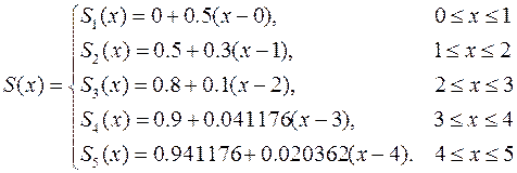
a)The slopes for all intervals can be computed (see Table 6.2), and the resulting first-order splines are:


b) Now fit quadratic splines to the same data using formulas:
 ;
;

Select  , then:
Hence,

c)The correct value of the function at x = 3.3 is f(x) = 0.915896.
d)The result of first-order splines at x = 3.3 is f(x) = 0.93. The percent relative error is εt = 1.5%. The result of quadratic splines at x = 3.3 is f(x) = 1.029706. The percent relative error is
εt = 12.4%.
Problems
1. Given the data:
| x | 2.5 | |||||
| f(x) |
Calculate f(4.4) using a) Newton (Gregory-Newton)interpolating polynomial, b) Newton's divided difference interpolating polynomial.
2. Employ inverse interpolating to determine the value of x that corresponds to f(x) =1.0 for the following tabulated data:
| x | 1.0 | 1.2 | 1.4 | 1.7 | 2.0 |
| f(x) | 0.5652 | 0.7147 | 0.8861 | 1.1964 | 1.5906 |
a) Use the linear splines; b) Use the Lagrange polynomial.
3. Develop cubic splines for the following tabulated data:
| x | |||||
| f(x) | 4.75 | 5.25 | 19.75 |
a)Calculate f(2.5) and f(4.0); b) Verify that S3(5) = S4(5).
COMPUTER LABS
"It is unworthy of excellent persons to lose hours like slaves in the labor of calculation."
– Gottfried Wilhelm von Leibniz
To the Student
Computers have been part of the landscape for some time now. The proliferation of mathematical software is changing the way that we use mathematics and programming, giving us the freedom to conduct numerical experiments without the drudgery of rote calculation. The payoff is that you'll learn to use a powerful tool, and develop numerical techniques without that would be difficult or impossible with pencil and paper alone.
Every student will do 5 laboratory works:
1. Numerical Integration.
2. Solution of linear algebraic equations.
3. Solution methods of non-linear equations.
4. Integration of ordinary differential equations.
5. Interpolation and extrapolation of functions.
In these assignments, you practice writing a few simple programs and compile them into executable programs using Pascal (C++) languages. If necessary, obtain a book (see some of the recommended ones in the SYLLABUS) and\or take a Pascal (C++) tutorial.
Make sure that your program is well commented/documented, structurally sound, aesthetically written, executes smoothly, and yields correct results. Submit both a hardcopy printout of the source code (program and results) and an executable file on a diskette for grading and discussing.
Date: 2016-01-14; view: 1313
| <== previous page | | | next page ==> |
| Part 5. Integration of Ordinary Differential Equations | | | Według klasyfikacji CIA |