CATEGORIES:
BiologyChemistryConstructionCultureEcologyEconomyElectronicsFinanceGeographyHistoryInformaticsLawMathematicsMechanicsMedicineOtherPedagogyPhilosophyPhysicsPolicyPsychologySociologySportTourism
For finding roots of algebraic and transcendental equations
| Method | Initial Guesses | Convergence Rate | Stability | Accuracy | Breadth of Application | Comments |
| Graphical | - | - | - | Poor | Real roots | May take more time than the numerical method |
| Bisection | Slow | Always | Good | Real roots | ||
| Secant | Medium to fast | Possibly divergent | Good | General | Initial guesses do not have to bracket the root | |
| False-position | Medium | Always | Good | Real roots | ||
| Newton-Raphson | Fast | Possibly divergent | Good | General | Requires evaluation of f¢(x) | |
| Newton-Raphson for Nonlinear Systems of Equations | n | Fast | Often diverge if the initial guesses are not sufficiently close to the true roots | Good | General | Requires evaluation of J(x) |
TABLE 4.2 Summary of important information
| Method | Formulation | Errors and Stopping Criteria |
| Bisection | 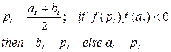
|  or or 
|
| Secant | 
|  or or 
|
| False Position |  ;
if ;
if 

| or
|
| Newton-Raphson | 
|  or or 
|
| Newton-Raphson for Nonlinear Systems of Equations | 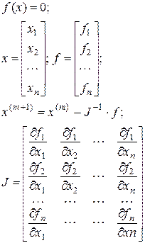
| 
|
Example 1
Determine the real root of  :
:
a)Graphically.
b)Using the bisection method (three iterations).
c)Using the secant method (three iterations).
d)Using the false position method (three iterations).
e)Using the Newton-Raphson method (three iterations).
Solution. a)The graphical approach for determining the roots of an equation.
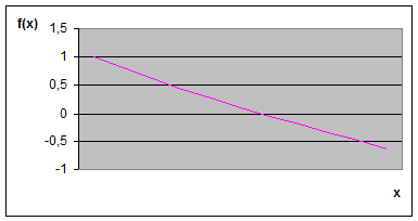 x x
| f(x) |
| 0.1 | 0.804837 |
| 0.2 | 0.618731 |
| 0.3 | 0.440818 |
| 0.4 | 0.27032 |
| 0.5 | 0.106531 |
| 0.6 | -0.05119 |
| 0.7 | -0.20341 |
| 0.8 | -0.35067 |
| 0.9 | -0.49343 |
| -0.63212 | |
The root is  .
.
b)Bisection method.
Using bisection, the results can be summarized as
| Iteration, i | ai | bi | xi | f(ai) | f(bi) | f(xi) |
| 0.5 | -0.63212 | 0.106531 | ||||
| 0.5 | 0.75 | 0.106531 | -0.63212 | -0.277633 | ||
| 0.5 | 0.75 | 0.625 | 0.106531 | -0.277633 | -0.089738 | |
| 0.5 | 0.625 | 0.5625 | 0.106531 | -0.089738 | 0.007283 |
Thus, after three iterations the root is x » 0.5625, f(x) = 0.007283 @ 0,  .
.
c)Secant method.
Use the secant method to find the root with initial estimates of  and
and  .
.
First iteration:


Second iteration:

Note that both estimates are now on the same side of the root.


Third iteration:


d)False position method.
Use the false position method with guesses of a0 = 0 and b0 = 1.
First iteration:


Second iteration:
Therefore, the root lies in the first subinterval, and p1 becomes:


 .
.
Third iteration:  .
.
Therefore, the root lies in the first subinterval:


e)Newton-Raphson method.
The first derivative of the function can be evaluated as
 which can be substituted along with the original function into equation (see table 4.2) to give:
 .
.
Starting with an initial guess of x0 = 1, this iterative equation can be applied to compute
| i | xi | f(xi) | ea, % |
| -0.63212 | |||
| 0.537883 | 0.0461 | 85.9 | |
| 0.566987 | 0.000245 | 5.1 | |
| 0.567143 | 4.541×10⁻⁸ | 2.8×10⁻² |
Thus, the method rapidly converges on the true root.
Notice that the percent relative error decreases at each iteration much faster than it does in another methods.
Example 2
Use the Newton-Raphson method for nonlinear system to determine the roots of equations:

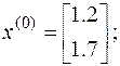
Solution. Graphical method gives us solution (point): M(1.2; 1.7). For this system Jacobian matrix is
 .
.
Hence, at the initial guesses we approximated roots as
 then
then 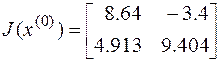 .
.
First iteration:
Thus, the determinant of the Jacobian for the first iteration is  . The values of the functions can be evaluated at the initial guesses as
  .
.
Hence,  . From the formula:

Check, how the results are converging to the true values:
 .
.
 .
.
Second iteration:
Repeat this process and we will have

The computation can be repeated until an acceptable accuracy is obtained.
Problems
1. Determine the real roots of  : (a)graphically, (b)using the Newton-Raphson method, and (c)using the secant method. Compare and discuss the rate of convergence.
2. Locate the first positive root of  . Use four iterations of (a)the bisection method, and (b)the false position method. Discuss and also perform an error check of your final answer.
3. Determine the roots of the nonlinear system of equations using the Newton-Raphson method:

Use graphical approach to obtain your initial guesses. Discuss and estimate the rate of convergence.
Date: 2016-01-14; view: 1220
| <== previous page | | | next page ==> |
| Part 3. Solution of Linear Algebraic Equations | | | Part 5. Integration of Ordinary Differential Equations |