A digital fountain's encoder

The encoding algorithm produces an droplet, v, from a number of source

segments. The number of source segments used to produce a droplet is

called the degree, and this is chosen at random from a previously determined

degree distribution.

This encoding operation defines a graph connecting encoded packets to source packets. If the mean degree is significantly smaller than K then the graph is sparse. We can think of the resulting code as an irregular low-density generator-matrix code.

For example, if the sender and receiver have synchronized clocks, they could use identical pseudo-random number generators, seeded by the clock, to choose each random degree and each set of connections. Alternatively, the sender could pick a random key, k_n, given which the degree and the connections are determined by a pseudorandom process, and send that key in the header of the packet. As long as the packet size l is much bigger than the key size (which need only be 32 bits or so), this key introduces only a small overhead cost.

A fatal flaw of maximum likelihood

Example:when we fit K = 4 means to our first toy data set, we sometimes find that very small clusters form, covering just one or two data points. This is a pathological property of soft K-means clustering, versions 2 and 3.

A popular replacement for maximizing the likelihood is maximizing the Bayesian posterior probability density of the parameters instead. However, multiplying the likelihood by a prior and maximizing the posterior does not make the above problems go away; the posterior density often also has infinitely-large spikes, and the maximum of the posterior probability density is often unrepresentative of the whole posterior distribution. Think back to the concept of typicality: in high dimensions, most of the probability mass is in a typical set whose properties are quite different from the points that have the maximum probability density. Maxima are atypical.

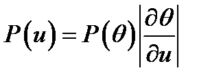
A further reason for disliking the maximum a posteriori is that it is basis-dependent. If we make a nonlinear change of basis from the parameter θ to the parameter u = f(θ) then the probability density of θ is transformed to

The maximum of the density P(u) will usually not coincide with the maximum of the density P(θ).

It seems undesirable to use a method whose answers change when we change representation.

A taste of Banburismus

The details of the code-breaking methods of Bletchley Park were kept secret for a long time, but some aspects of Banburismus can be pieced together.

How much information was needed? The number of possible settings of the Enigma machine was about 8×10¹². To deduce the state of the machine, `it was therefore necessary to find about 129 decibans from somewhere', as Good puts it. Banburismus was aimed not at deducing the entire state of the machine, but only at figuring out which wheels were in use; the logic-based bombes, fed with guesses of the plaintext (cribs), were then used to crack what the settings of the wheels were.

The Enigma machine, once its wheels and plugs were put in place, implemented a continually-changing permutation cypher that wandered deterministically through a state space of 26³ permutations. Because an enormous number of messages were sent each day, there was a good chance that whatever state one machine was in when sending one character of a message, there would be another machine in the same state while sending a particular character in another message.

Date: 2015-01-29; view: 867