CATEGORIES:
BiologyChemistryConstructionCultureEcologyEconomyElectronicsFinanceGeographyHistoryInformaticsLawMathematicsMechanicsMedicineOtherPedagogyPhilosophyPhysicsPolicyPsychologySociologySportTourism
Systematic convolutional codes correcting capability research
Objective: To determinate the quality parameters of the system with the error-correction coding by convolutional code (14, 7) with a threshold algorithm decoding in a channel with additive white Gaussian noise (AWGN).
Laboratory emulator:
After opening the file “Project1.exe” you can see interface like fig. 3.6.

Figure 3.6 – The interface of laboratory work
You need enter the data from table 3.6, where p0 – error probability, L – amount of codewords.
Table 3.6 – Results of coding gain by error probability in the DSC
| p0 | 0,07 | 0,05 | 0,03 | 0,01 | 0,005 | 0,003 |
| L | 25·104 | 5·105 | 75·104 | 106 | 4·106 | 5·106 |
| Wep |
In the result of the experiment, you get next parameters:
- i1 – amount of errors in the discrete symmetric channel (DSC);
- i2 – amount of uncorrected errors by the decoder;
- k0 – errors coefficient in the DSC, k0 nearly equal p0;
- kd – errors coefficient in the output of the decoder;
- W – coding gain.
These parameters are calculated by formulas:
k0=i1/2L, kd =i2/L, W= k0/kd.
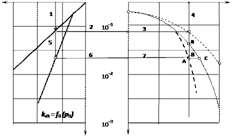
Then you can get the diagram kd1 = f0(p0)after putting the button “Построить график”, as shown in fig. 3.7a.
For building of the diagram for determination of coding gain W in the channel with AWGN it is need to use two subsidiary diagrams in the fig 3.7b. The first diagram is the characteristic of the channel with PM-2 without coding  . The second diagram
  with the double energy of the bit (as the relative information transfer rate R = ½).
p0 10–3 10–2 Р01 10-1 100 0 1 2 h1 3 h
 |
p0 = f2(  h)
h)
kd =p0
kd2= f3 (  h)p0=f1(
  h)
h)
kdkd, p0
а) b)
Figure 3.7 – The characteristic of the DSC and the channel with AWGN
For example, for given value p01 we can determinate the signal/noise ratio h1 using the path 1→2→3→4. The value h1 corresponds to error probability p01 in the output of the PM-2 demodulator. Take to account that there is convolutional decoder (14, 7) before PM-2 demodulator, which decreases error probability p0 in W times. That’s why the place of the point A on the diagram kd2 = f3(  h) is determined using the paths 1→5→6→7and 4→8. For getting the characteristic kd2 it is need to use some values of p0.
Laboratory task:
1. To open the file “Project1.exe”.
2. To enter initial data from the table 3.6 and fill it.
3. To draw the characteristic kd1 = f0 (p0).
4. To build the graph kd2 = f3(  h) using the values p0 from the table 3.6.
5. To determine the value hlim when the convolutional code (14, 7) is reasonable.
Home task:
1. To learn items 1.3.1 – 1.3.2 of this teaching manual.
2. To write down the answers to the general questions.
3. To prepare the table 3.6 in the protocol.
4. To prepare blank using Application B.
General questions:
1. What does the characteristic kd1 = f0 (p0) describe?
2. What does the characteristic kd2 = f3(  h) describe?
3. Determinate the coding gain by error probability Wep = p3/p4, where p3 – error probability in the channel without coding, p4 – with coding, if h = 2,1 and 2,3 using the diagram 3.7b.
Protocol content:
1. Subject and objective.
2. Executed home task.
3. Graph and table according to laboratory task.
4. Conclusion. Compare two characteristics of kd1 = f0(p0) and kd = f(p0) from the laboratory work 2.
Laboratory work 5
Date: 2016-01-14; view: 1031
| <== previous page | | | next page ==> |
| Cyclic codes correcting capability research | | | Nonsystematic convolutional codes correcting capability research |