CATEGORIES:
BiologyChemistryConstructionCultureEcologyEconomyElectronicsFinanceGeographyHistoryInformaticsLawMathematicsMechanicsMedicineOtherPedagogyPhilosophyPhysicsPolicyPsychologySociologySportTourism
Part 2. Numerical Integration
TABLE 2.1 Important integration formulas
| Method | Formula | Error |
| Left Sum Approximation | 
| ~O(h) |
| Right Sum Approximation | 
| ~O(h) |
| Midpoint Approximation | 
| ~O(h2) |
| Trapezoidal Approximation | 
| ~O(h2) |
| Simpson’s (1/3) Approximation | 
| ~O(h4) |
| Simple Monte Carlo Approximation | 
| ~ 
|
*  ; **
; **  .
.
Example 1
Suppose we want to evaluate the integral  . The definite integral is the area under the curve
  , above the x-axis and between the lines x = 0 and x = 10. The actual value can be easily obtained as follows:

 .
.
Solution. n = 4(h = 2.5)

a)Use it in conjunction with Left sum approximation to integrate the same function for four subintervals:
 .
.
The numerical error and the true percent relative error are:
 .
.
b)Using Right sum approximation:
 .
.
 .
.
c)Using Trapezoidal Rule (four subintervals):
 .
.
 .
.
d)Using Simpson's 1/3 Rule (four subintervals):
 .
.
 .
.
Example 2
Suppose we want to evaluate the following double integral:
 .
.
For the numerical evaluations use both the trapezoidal and Simpson's 1/3 rules. For both cases, use the multiple-application version, with n = 4. Compute percent relative errors for the numerical results.
Solution.
a) Analytically the actual value can be easily obtained as follows:

b)Numerical integration with n = 4:(hx = 1.0; hy = 2.0)

c)Use it in conjunction with Trapezoidal Rule to integrate the same function for four subintervals:

 .
.
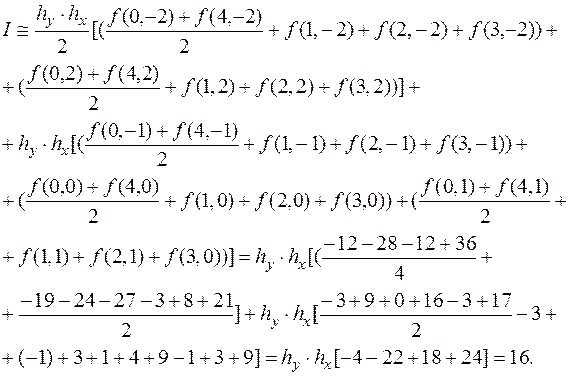
d)Using Simpson's 1/3 Rule:

 .
.
Note:
· Trapezoidal rule gives the exact value of the integral for linear polynomials;
· The Simpson's rule gives the exact value of the integral for polynomials of degree three or less;
· An even number subintervals must be utilized to the Simpson's rule;
· As the number of subintervals increases, the approximations get better.
Problems
1. Integrate the following function both analytically and numerically.
 .
.
For the numerical evaluations use: (a) left sum approximation,
(b)right sum approximation, and (c)midpoint approximation. For all cases use version with n = 4. Compute percent relative errors for the numerical results.
2. Integrate the following function:
 .
.
Note that the true value is I = 0.602297. Use both the trapezoidal and Simpson's 1/3 rules to numerically integrate the function with n = 4.
3. Evaluate the triple integral

(a) analytically, and (b)using Simpson's 1/3 rule with n = 4.
For (b)compute the percent relative error (  ).
).
4. Integrate the following function both analytically and numerically.
 .
.
For the numerical evaluations use: (a) midpoint approximation,
(b)Monte Carlo integration.
A random sample (  ) of size 20 is given below:
| i | 
| i | 
| i | 
| i | 
|
| 0.0105 | 0.2171 | 0.2747 | 0,4150 | ||||
| 0.0039 | 0.5369 | 0.4442 | 0.1651 | ||||
| 0.3351 | 0.1957 | 0.1089 | 0.8154 | ||||
| 0.0332 | 0.7003 | 0.6982 | 0.6855 | ||||
| 0.3557 | 0.9498 | 0.5643 | 0.7643 |
For all cases use version with n = 10. Compute percent relative errors for the numerical results. Discuss your results.
5. The function

can be used to generate the following table of unequally spaced data:
| x | 0.0 | 0.12 | 0.22 | 0.32 | 0.36 | 0.40 | 0.44 | 0.54 |
| f(x) | 0.20000 | 1.309729 | 1.305241 | 1.743393 | 2.074903 | 2.456000 | 2.842985 | 3.507297 |
Evaluate the integral from a = 0 to b = 0.54 using: (a)analytical means, (b)left sum approximation, (c)right sum approximation, and (d)the trapezoidal rule. For (b), (c)and (d),compute the percent relative error (  ).
).
Date: 2016-01-14; view: 3313
| <== previous page | | | next page ==> |
| Contents of the Course | | | Part 3. Solution of Linear Algebraic Equations |