CATEGORIES:
BiologyChemistryConstructionCultureEcologyEconomyElectronicsFinanceGeographyHistoryInformaticsLawMathematicsMechanicsMedicineOtherPedagogyPhilosophyPhysicsPolicyPsychologySociologySportTourism
Introduction to Polymer Science and Technology
Mechanical properties
 60 80 100
strain (s), %
Figure 6.7Stress-strain curves for HIPS at a range of temperatures from -40 °C to 80 °C (tests conducted at 2 mm/min cross-head speed) (source:
Ehrenstein(2001,p182)
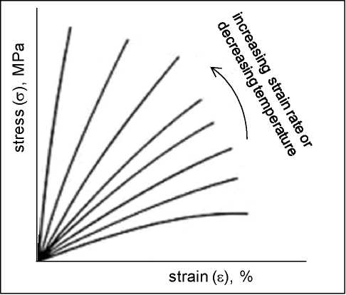
Figure 6.8Illustration of the effect of temperature and speed of deformation on stress-strain behaviour of polymeric materials
6.2.2 Effect of water absorption
Water absorption should be a particular consideration for hygroscopic polymers. Many engineering polymers such as polyamides (nylons), ABS, polycarbonate, cellulosics, and poly(methyl methacrylate). Other polymers, e.g., polyethylenes and polystyrene, do not normally absorb much moisture, but are able to carry significant moisture on their surface when exposed to water. Table 6.2 lists the water absorption values for several selected plastics as determined by ASTM D 570 after 24 h immersion at 23 °C. Equilibrium value for water absorption will be significantly higher for these plastics, as will water absorption values obtained at elevated temperatures (BASF-1, 2003).
Introduction to Polymer Science and Technology
Mechanical properties
Table 6.2Water absorption values for selected plastics
| Polymer | Water absorption, % |
| polypropylene | <0.01 |
| polycarbonate | 0.15 |
| nylon 11 | 0.25 |
| nylon 6 | 1.3 |
| cellulose acetate | 1.7 |
Polyamides are widely used engineering materials and their water absorption has received wide coverage, e.g., Akay (1994). CAMPUS provides comprehensive data on this subject.
Figure 6.9 shows the effect of moisture on polyamide 66: as can be seen, increasing moisture content results in lowering of Youngs modulus (greater flexibility) and the yield and tensile strengths but also an increase in ductility (i.e., % elongation to failure) and toughness (as indicated by the area under the stress-strain curve).

|
 Q_
Q_
CO CO
CO
I l
Dry as moulded
0,2% moisture content"
EQ% RH -123% moisture content]
100% RH
[8,5% moisture content)
0 50 100 150 200 250 300
strain, %
Figure 6.9Room temperature tensile stress-strain curves for PA66 specimens with various moisture contents (source: DuPont Handbook on nylon
resins, p3.1)
The extent of moisture absorption is accelerated with temperature, and obviously under hygrothermal conditions the properties suffer much greater deterioration, see Figure 6.10.
Introduction to Polymer Science and Technology
Mechanical properties
| -40 |
| i, MPa | |
| j_ ^) г— | |
| CD | |
| "So | |
| Id |
| ч \ | \ | ||
| \ \ | \ V | ||
| \ | |||
| — —__ |
40 80 120
temperature, °C
Figure 6.10Yield strength vs. temperature for PA66 specimens with various moisture contents (source: DuPont Handbook on nylon resins, p3.1)
Introduction to Polymer Science and Technology
Mechanical properties
6.2.3 Effect of long-term loading
Viscoelastic materials will suffer gradual deformation under small loads (corresponding to below yield strength) even at room temperature. Thermoplastics, in general, are more prone than thermosets to time-dependant deformation under a given load. The long term stress-strain behaviour is described in terms of either creep (on one occasion when I was covering the subject of creep, a student who spent 6 years to get his HND in Engineering and became a good musician whispered, "a bit of a creep yourself" when the subject was dragging on a bit!) or stress relaxation (which was my response!). Creep is measured by applying a constant load (constant engineering stress) to a specimen and measuring deformation over time. Conversely, in stress relaxation the material is subjected to a constant strain and the stress to maintain this strain is recorded over time.
Creep data (i.e., strain vs. time) is usually obtained for different levels of stress and, it may also be necessary to obtain data at different temperatures. The data is of significance particularly for brittle plastics that can only support limited strain to failure. From a set of creep strain vs. time data isochronous stress-strain curves and stress relaxation curves (isometric curves) can be constructed as illustrated in Figure 6.11. Similar to an isometric curve, a creep modulus (E(t) = a(t) / e') vs. time curve can also be presented from the ratios of stress to strain at a given strain

Figure 6.11Construction of a creep isochronous o-s curve (c) and an isometric stress-time curve (b) from creep curves (a). (Isochronous indicates the same time period, and isometric indicates equal measure, here the same strain)
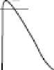
Isochronous curves for various polymer types and by various producers are presented in the Material Data Centre web site (www.materialdatacenter.com) as shown in Figure 6.12 for PA66.
Introduction to Polymer Science and Technology
Mechanical properties
|
Figure 6.12ст-s isochronous curves for Zytel 101L NC010 (PA66) (cond.) at 23 °C
Temperature dependence of processes such as creep, stress relaxation as well as ageing can be described by the Arrhenius equation,see below, which produces a straight line when the loge(change in property) is plotted against 1/T.
The process rate (T) = Ae(Q/RT) where, Q is the activation energy, R is the gas constant, T is the absolute temperature, and A is a pre-exponential constant.
Creep is normally determined under tensile loading for plastics, but there are also standard test methods for creep in flexure. However, creep tests for elastomers are usually conducted in compression and also in shear. The differences reflect the type of applications that these materials are employed for. Stress relaxation tests are normally conducted in tensile deformation mode, but rubber and other materials that are used as seals or gaskets are tested in compression.
The Boltzmann superposition principle,an aspect of linear viscoelasticity, considers the entire loading history of deformation: it states that deformation over time, e(t), is dependent on the entire loading history of the material in the form of independent, discrete loading steps (these may be positive (added) or negative (removed). Accordingly, creep after a period of time, t, due to many discrete/incremental (step) loads, Дстр A ст2, A ст3, ... , A стп, applied at times ui; u2,u3, ... ,un, becomes the sum of the contributions of every loading step:
e(t) = Act J(t - u) + Act J(t - u) + Act J(t - u)
Act J(t - u) or
where, J(t) is the creep compliance, i.e., J(t) = 1 / E(t).
Introduction to Polymer Science and Technology Mechanical properties
If the stress changes continuously, the superposition principle can be expressed in an integral form and gives the creep deformation as t
U=—со
or more correctly
where, u is the time variable and integration covers the whole stress history, i.e., (- со < u 5= t), and aQ/E0 represents the initial elastic deformation
6.3 Flexural properties
Materials can undergo flexing or bending in their applications, which is replicated in the form of three-point bending, four-point bending and cantilever bending in testing, see Figure 6. 13. The three- and four-point bending tests are popular because of the simplicity of test pieces and also the avoidance of clamp-gripping problems associated with tensile testing. The standard methods for conducting flexural tests for plastics include ISO 178:2010 or BS 2782-3: Method 335A for three-point loading test. ASTM D790M-10 describes methods for both modes of loading, and ASTM D6272-10 standard test method is for four-point bending. ASTM D747 - 10 covers the determination of the apparent bending modulus of plastics by means of a cantilever beam bending. It is useful for materials that are too flexible to be tested by other standard methods.
Introduction to Polymer Science and Technology
Mechanical properties
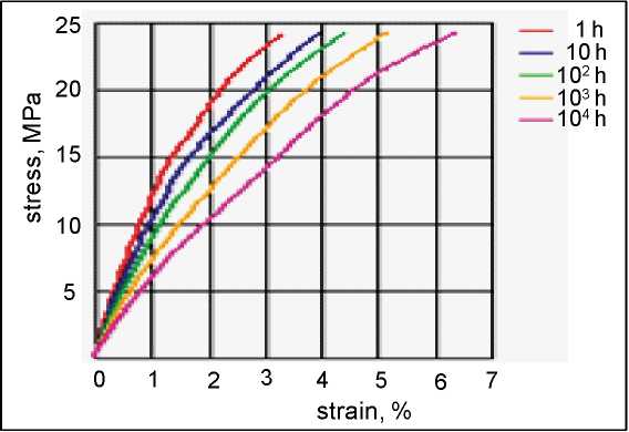
Figure 6.13Flexural modes: (a) 3-point bending, (b) 4-point bending, (c) simple cantilever
The tests are conducted using rectangular-bar test pieces of certain dimensions on a universal test machine with suitable loading fixture (Figure 6.14).

Figure 6.14A specimen tested in 3-point bending
For three- and four-point bending tests, the test pieces are supported on cylindrical surfaces and loaded centrally via a rounded loading nose(s) of certain diameters. The diameters are selected to avoid too much indentation and premature failure due to stress concentration under the loading nose(s). Three- point bending tests are commonly used, but in the four-point bending mode the stress is distributed over a wider span surface between the inner loading noses and, therefore, becomes more uniform rather than concentrated under the loading nose in three-point bending. Four-point bendingis useful in testing materials that do not fail at the point of maximum stressin three-point bending.
ISO 178:2010 specifies two methods, Method A and Method B. In Method A, a strain rate of 1 %/min is used throughout the test. Method В uses two different strain rates: 1 %/min for the determination of the flexural modulus and 5 %/min or 50 %/min, depending on the ductility of the material, for the determination of the remainder of the flexural stress-strain curve. A variety of specimen shapes can be used for this test, but the most commonly used specimen size for ASTM is 3.2 x 12.7 x 127 mm and for ISO is 4 xlO x 80 mm in thickness (depth), width and length, with a support span-to-depth ratio of 16. This should provide sufficient overhang to prevent the specimen from slipping through the supports during the test.
Introduction to Polymer Science and Technology
Mechanical properties
The stress and strain are not uniform through the specimen thickness: during loading the stress and strain varies gradually from a maximum compressive form on the surface in contact with the loading nose(s), through zero at the neutral plane, to a maximum tensile form on the outer surface. The maximum axial fibre stresses occur on a line under the loading nose in 3-point bending and over the area between the loading noses in 4-point bending. It is the maximum tensile stress and strain that are computed. The outcome of a test is usually a plot of load versus displacement, see Figure 6.15.
Various flexural properties can be calculated by extracting data from these plots and using the equations presented below, such as flexural modulus (modulus of elasticity in flexure), flexural strength (also known as 'modulus of rupture' when maximum stress in the outer fibres at the moment of break is recorded). Other flexural properties include yield strength, strain at yield, offset yield strength (the stress at which the stress-strain curve deviates by a given strain (offset) from the tangent to the initial straight line portion of the stress-strain curve), flexural stress at 3.5% deflection (ISO) (deflection equals to 1.5 times the thickness of the test specimen) or 5.0% deflection (ASTM), and secant modulus of elasticity (i.e., the slope of the straight line that joins the origin and a selected point on the actual stress-strain curve).

Figure 6.15A load vs. deflection plot from 3-point bending test of a wood-plastic specimen
The equations, see the standards, for the flexural stress (maximum fibre stress) (of) and strain (ef) for a rectangular-bar test piece under three-point loading are given as
af=(3FL)/(2bh2);£f=(6hs)/(L2)
where, F is the force at midspan, L is the support span, h the specimen thickness, b the width and s is the deflection of the tensile surface of the specimen at midpoint.
The modulus of elasticity (Ef), from the above equations, becomes
Ef= [L7(4bh3)] x (slope)
Introduction to Polymer Science and Technology Mechanical properties
where , 'slope ' is the slope of the tangent to the initial straight-line portion of the load-deflection curve.
The equations for a rectangular-bar test piece under four-point loading, where the load span (the distance between the two loading noses) is one third of the support span are given as
af=(FL)/(bh2);£f=(4.7hs)/(L2) .-. Ef= [0.21L7(bh3)] x (slope) There are equivalent equations for cylindrical test pieces.
In theory, the flexural modulus and the tensile modulus should be the same. However, as described by Hawley (1999, p320), in practice this is only approximately so, because plastic test pieces are not isotropic through their thickness. Differential cooling rates, variations in extrusion or injection rates and changes in flow patterns, all contribute to non-uniform microstructure and properties across the thickness. When coupled with non uniform stresses in flexural testing, mentioned above, that inconsistencies with tensile test can arise.
Table 6.3 shows single-point flexural data (obtained under standard laboratory conditions of approximately 23 °C and 50 % relative humidity in 3-point bending, and mostly in accordance with ASTM D790) for dry-as-moulded samples. The table, as in Table 6.1, include the most quoted value and the minimum and maximum values in brackets.
Introduction to Polymer Science and Technology
Mechanical properties
Table 6.3Flexural properties of various polymers (sources: CAMPUS, Efunda, Plastics International
| Polymer type | Abbrn. | Flexural modulus, GPa | Flexural strength, MPa | Compressive modulus, GPa | Compr. strength, MPa | Compr. yield strength, MPa |
| Commodity thermoplastics | ||||||
| Low-density polyethylene | LDPE | 0.2-0.3 | ||||
| High-density polyethylene | HDPE | 1-1.6 | 19-25 | |||
| Polypropylene | PP | 1.5(1.2-1.7) | 48 (40-55) | 1.6(1.1-2.1) | 38-55 | |
| Polystyrene | PS | 2.5-3.4 | 70(69-101) | 3.3-3.4 | 83-90 | |
| Polyvinyl chloride (rigid) | PVC | 1.4-3.5 | 41-110 | 2.6 | 55-90 | |
| Styrene-acrylonitrile copolymer | SAN | 3.5-4.2 | 76-131 | 3.7-4 | 97-104 | |
| Engineering thermoplastics | ||||||
| Acrylonitrile-butadiene-styrene copolymer | ABS | 2.5(2.1-2.8) | 75( 49-90) | 1.4-3.1 | 86 (12-86) | |
| Polyamide6,6 | PA 6,6 | 2.8 (2.8-3.2) | 110 (12-124) | 35-104 | ||
| Polybutylene terephthalate | PBT | 2.3 (2.3-2.8) | 83(83-115) | 2.6 | 59-100 | |
| polycarbonate | PC | 2.3 (2-2.4) | 90(71-103) | 2.4 | 69-86 | |
| Polyethylene terephthalate | PET | 2.8(2.4-3.1) | 80-114 | 76-104 | ||
| Polymethyl methacrylate | PMMA | 3 (2.2-3.2) | 100(72-131) | 2.6-3.2 | 72-124 | |
| Polyoxymethylene (acetal) | POM | 2.8 (2.6-3.4) | 97(94-110) | 4.6 | 108-124 (at 10% strain) | |
| Polyurethane | PU | 2(1.3-2.1) | 100 (70-104) | |||
| Ultrahigh molecular weight polyethylene | UHMWPE | 0.9-1.0 | 0.52 | |||
| High-performance engineering thermoplastics | ||||||
| Polytetrafluoroethylene (a fluoropolymer) | PTFE | 0.5 | 0.41 | 7-12 | ||
| Polyphenylene oxide (impact modified) | PPO | 2.4 (2.3-2.8) | 95 (66-97) | |||
| Polyetherether ketone | PEEK | 3.6-4 | 110-170 | 3.8 |
Introduction to Polymer Science and Technology
Mechanical properties
| Polyetherimide | PEI | 3.3 | 3.3 | |||
| Polyethersulphone | PES | 2.6 | 2.7 | |||
| Polyimide | PI | 3 (2.5-3.5) | 140 (69-199) | 2.2-2.4 | 121-276 | |
| Polyphenylene sulphide | PPS | 3.8(3.8-4.1) | 96(96-145 | |||
| Polysulphone | PSU | 2.6-2.7 | 106-121 | 2.6 | ||
| Thermosets | ||||||
| Epoxy resin | EP | 2.5-2.9 | 90-145 | 104-173 | ||
| Melamine-formaldehyde (cellulose filled) | MF | 7.6 | 62-110 | 228-311 | ||
| Phenol-formaldehyde | PF | 76-117 | 83-104 | |||
| Polyester (unsatu rated) resin (rigid) | UP | 3.0 (3.0-4.2) | 100 (59-159) | 90-207 | ||
| Polyimide resin | PI | 4 (2.9-20) | 176 (45-345) | 2.9 | 133-227 | |
| Polyurethane (casting) | PU | 4.2 |
6.4 Compressive properties
Plastics are subjected to compression in use, mainly as elastomeric materials and cellular plastics. Compression generates various degrees of bulging/barrelling and buckling in materials depending on the shape and size of the component and the rigidity of the material. Bulging and emaciation, depending on the mode of deformation, enables the volume of elastomers to remain constant, which is why their Poissons ratio is approximately 0.5. The thickness of an elastomeric block dictates its stiffness under compression: a thin block will not bulge as much as a thick block and, therefore, exhibit greater stiffness. The influence of thickness on stiffness can be expressed in terms of a parameter known as the shape factor, S, such that the compression modulus, Ec, for a block of an elastomer in terms of Youngs modulus, E, and shape factor becomes
Ec =
2S2).
S is defined as the ratio of loaded area to force-free area (bulge-prone area). Accordingly for a normal rectangular block of sides a, b and с (the height or the thickness), S = (ab)/[2c(a + b)]. Hence as the thickness decreases, S increases.
In rigid and semi-rigid plastics, buckling is of concern and the standard methods for conducting compression tests for plastics, ISO 604: 2002 or BS 2782: Method 345A and ASTM D695M-10, specify test pieces and fixtures to avoid buckling. In specimens prone to buckling, the specimen length may be further adjusted. Specimens recommended are rectangular prisms of 4 x 10 mm in cross section and of 10 mm length for strength and 50 mm length for elastic modulus determinations. Smaller dimensions are also specified to allow for restrictions due to the amount of material available or geometric constraints on a product/component. Normally the specimens should be conditioned and the tests should be conducted in a standard room atmosphere of 23/50.
Introduction to Polymer Science and Technology
Mechanical properties
During the test, force and the corresponding compression data is recorded. Therefore, at the outcome of the test, a plot of force vs. compression or more commonly stress vs. strain is produced, see Figure 6.16.
stress (a), MPa

|
scy scx scb - scm scm scb strain (e), %
Figure 6.16Typical compressive stress-strain curves (source: ISO 604:2002)
Introduction to Polymer Science and Technology Mechanical properties
Various compressive properties can be calculated by extracting data from these plots and using the equations indicated under Section 6.2 for tensile properties. The properties include compressive modulus (e.g., modulus of elasticity in compression), compressive strength, o"cM (maximum stress sustained by the specimen during the test) or o"cB (stress at break). Other properties include strain to break and/or to reach maximum stress, £cB, £cM; stress and strain at yield, o"cY> £cY, stress at a certain % strain, o"cX, etc. The values of some of these properties for some polymers are included in Table 6.3.
6.5 Shear properties
Testing for shear properties of strength and shear modulus is not so common for ordinary plastics; it is used more for elastomeric and composite materials. The standard test methods for plastics are BS 2782-3 Methods 340A and В and ASTM D732-10 for determination of shear strength by punch tool.
The specimens are in the form of disks, square plaques or rectangular bars of specified dimensions. In testing, the specimen is clamped between the two halves of an annular clamp. A round punch type of piston that fits the opening in the clamp is bolted to the specimen, and a load is applied to the specimen via the punch to push it through the clamp at such a rate that specimen fractures within 15 to 45 s. The shear strength, t, is calculated as the maximum force encountered during the test divided by the area of the sheared edge. Therefore, for a specimen that is bolted to the punch,
xs = F / (ttDT) where, F is the force at break, D is the punch diameter and T is thickness of the specimen.
ISO 1827:2007 specifies methods for the determination of modulus in shear and adhesion strength to rigid plates for vulcanized or thermoplastic rubber, using four pieces of rubber bonded/sandwiched between four parallel plates (quadruple-shear method). Other approaches employ test pieces that consist of one-lap (a rubber layer between two metal plates) or two-lap (two layers of rubber between three metal plates) shear units.
Shear modulus, G, is determined at small strain levels where the stress-strain relationship is linear (i.e., elastic) using the equation G = т / у, where т and у are shear stress and strain, respectively.
The elastic moduli properties obtained under different loading modes are related to each other through the constant of Poissons ratio, v, for example
E = 2(1 + v) G. Therefore, together with Youngs, the shear and the bulk moduli, Poissons ratio becomes one of the four elastic constants.
The Poissons ratio of isotropic, linear elastic solids cannot be less than -1 nor greater than 0.5, since moduli terms have positive values. However, it is rare to encounter engineering materials with negative Poissons ratios: for most materials, it will fall in the range of 0.0 and 0.5. The Poissons ratio for most metals is approximately 0.3. Rubber has a Poissons ratio close to 0.5 and is therefore almost incompressible. Cork has a Poissons ratio close to zero, showing very little lateral expansion when compressed and, therefore, functions well as a bottle stopper since it will not swell laterally when pushed into a bottle.
Introduction to Polymer Science and Technology Mechanical properties
Some polymer foams have a negative Poissons ratio; if these auxetic materials are stretched in one direction, they become thicker in perpendicular directions. Some anisotropic materials have one or more Poissons ratios above 0.5 in some directions.
6.6 Hardness
Hardness is a measure of the level of penetration of an indentor when forced into the material under specified conditions, although the term hardness has been applied to scratch resistance and to rebound resilience as well. Brown (1999, p 226) describes the mode of deformation under an indentor as a mixture of tension, shear and compression, and not a fundamental material property. The indentation hardness is inversely related to the extent of penetration and is dependent on the elastic modulus and viscoelastic behaviour of the material. Empirical equations relating applied load, depth of indentation and indentor geometry to modulus of elasticity for different indentor geometries are presented by Brisco et al. (1994).
Hardness as a material property is used more in association with elastomers than with plastics. The results depend on the indentor geometry, the extent of indentation as well as the delay between the application of the indentor and when the hardness is recorded. Regardless of the arbitrary nature of the test, it is attractive because of its cheapness, simplicity, and applicability to finished components as well as specimens, and it is virtually a non-destructive test.
The standard test methods for plastics and rubbers are ISO 868: 2003, BS 2782-3 Method 365B and ASTM D2240-05 for determination of indentation hardness by means of a Shore durometer. The Shore hardness tester is a hand-held simple device consisting of a needle-like spring-loaded indentor, which is pressed into the specimen surface and the penetration of the needle is measured directly from a scale on the device in terms of hardness degrees. There are two types of Shore durometers with different levels of indentor stiffness; Shore A Durometer is fitted with a blunt indentor and is suitable for soft elastomers and plastics and Shore D, with a sharper-tipped indentor, for harder elastomers and plastics.
Alternative standard test methods recommend hardness testers with spherical indentors. These are ISO 2039-1: 2001, BS 2782-3 Method 365D and ASTM D2240-05. In ball indentation, the hardness is expressed in terms of the surface area of the impression left on the surface of the material by the indentor following the test, rather than the penetration of the indentor.
The Rockwell hardness tester is another ball indentation method, described in ISO 2039-2: 2001 and ASTM D785, however, here the hardness is expressed in terms of the penetration of the indentor. The method is suitable for harder thermoplastics and thermosets, and depending on the load applied and the ball diameter used different Rockwell hardness scales are defined. Table 6.4 shows a range of hardness values for various polymeric materials over hardness scales of Shore A, Shore D or Rockwell R and M.
Introduction to Polymer Science and Technology
Mechanical properties
Table 6.4Hardness properties of various polymers (sources: ASM International (2003), Efunda)
| Polymer type | Specific gravity | Hardness | ||||
| Shore A | Shore D | Rockwell R | Rockwell M | Barcol | ||
| Commodity thermoplastics | ||||||
| LDPE | 0.92(0.91-0.93) | 44-50 | ||||
| HDPE | 0.95 (0.94-0.96) | 66-73 | ||||
| PP | 0.9 (0.9-0.95) | 80(80-102) | ||||
| PS | 1.1 | 60-75 | ||||
| PVC | 1.4(1.38-1.55) | 65-85 | ||||
| SAN | 1.08 | 75-83 | ||||
| Engineering thermoplastics | ||||||
| ABS | 1.05(1.03-1.07) | 102-115 | ||||
| PA 6,6 | 1.15(1.07-1.24) | |||||
| PBT | 1.31 (1.30-1.38) | 68-78 | ||||
| PC | 1.2(1.06-1.25) | 70 (62-75) | ||||
| PET | 1.37(1.33-1.48) | 94-101 | ||||
| PMMA | 1.2(1.17-1.23) | 68-105 | ||||
| POM | 1.41 (1.4-1.54) | 92-94 | ||||
| PU | 1.16(1-1.24) | |||||
| TPU | 1.20-1.25 | 55-94 | ||||
| UHMW-PE | 0.94 | 61-63 | ||||
| High-performance engineering thermoplastics | ||||||
| PTFE | 2.13(2.1-2.35) | 50-65 | ||||
| PPO | 1.06 | 115(94-120) | ||||
| PEI | 1.27 | |||||
| PES | 1.37 | |||||
| PI | 1.4 | 95; E(52-99) | ||||
| PPS | 1.34(1.3-1.35) | 123(120-125) | ||||
| PSU | 1.24 | |||||
| Thermosets | ||||||
| EP | 1.4(1.1-1.9) | 80-110 | ||||
| MF | 1.5 | 120(115-125) | ||||
| PF | 1.32(1.24-1.4) | 110(93-120) | ||||
| UP | 1.5(1.2-2) | 40 (34-75) | ||||
| PI | 1.43 | 110-120 | ||||
| PU | 1.05 | 50-70 | 30-35 | |||
| UF (cellulose filled) | 1.5 | 110-120 |
Introduction to Polymer Science and Technology Mechanical properties
Hardness test methods that are normally used for metals, but are also used in characterising plastics, include Brinell and Vickers.
6.7 Impact properties and fracture toughness
Under impact, material is subjected to a sudden blow of a projectile or a hammer. The speed of impact testing is much higher than the strain rates encountered in the tests covered previously, which are classified as static tests. Impact tests can be conducted in the form of pendulum tests, falling mass (dart) tests and high speed tensile tests. The basic equipment at best indicate the energy absorbed in the process of specimen fracture, however, there are sophisticated equipment that are suitably instrumented to provide force-deflection traces from which more information can be gleaned as well as overall energy value at fracture.
Pendulum impact tests can be conducted in the mode of Charpy or Izod tests.
6.7.1 Charpy test
The standard test methods that describe the non-instrumented Charpy impact test include BS EN ISO 179-1: 2010 and ASTM D6110-10. Test pieces in the form of a rectangular bar maybe un-notched or contain a notch centrally cut into the test piece. The notch generates stress concentration in a simulation of real application conditions. As illustrated in Figure 6.17, the specimen is supported at both ends and is struck centrally by the pendulum head at the bottom of its swing. The specimens maybe tested in an edgewise or flatwise direction with respect to the impactor head. The edgewise positioning is the common practice for notch containing specimens. The ISO test pieces are 80 x 10 x 4 mm in dimension, with 2 mm depth notches of different notch-tip sharpnesses.
Introduction to Polymer Science and Technology
Mechanical properties

|
| striker |
| impact |
| end of swing' |
| specimen |
Figure 6.17Illustration of Charpy impact test (source: The Welding Institute)
The preferred notch-tip radius is 0.25 mm, however in order to determine notch sensitivity of the material, test pieces with the sharper (0.1 mm radius) and blunter (1.0 mm radius) notches are also tested. The standard specimen for ASTM is 64 x 12.7 x 3.2 mm, and the notch depth is 2.5 mm (i.e., the depth under the notch of the specimen is 10.2 mm)
ISO impact strength is calculated by dividing impact energy with the specimen cross-sectional area behind the notch and is expressed in J/m2. ASTM impact energy is calculated by dividing impact energy in J with the thickness of the specimen (i.e., the notch width) and is expressed in J/m.
6.7.2 Izod test
The standard test methods that describe the Izod impact test include ISO 180: 2000 and ASTM D256-10. As illustrated in Figure 6.18, the specimen is clamped at one end as a vertical cantilevered beam with the notched side facing the striking head of the pendulum; and its free half is struck centrally by the pendulum head at the bottom of its swing. The dimensions of the test pieces are the same as for the Charpy test and the impact strength is also expressed similarly.
Charpy and Izod tests are suitable for plastic specimens that offer sufficient rigidity to avoid buckling, for specimens that are not sufficiently thick or materials that undergo high elongation to failure the tensile impact test is recommended, see ISO8256:2004 and ASTM D1822M-93.
Table 6.5 shows a range of notched impact values for various polymeric materials (obtained under standard laboratory conditions of approximately 23 °C and 50 % relative humidity on dry-as-moulded samples).
Introduction to Polymer Science and Technology
Mechanical properties

Figure 6.18Illustration of Izod impact test
Table 6.5Impact properties of various polymers (sources: Efunda, Plastics International, CAMPUS, Ehrenstein (2001, p260), Fried (1995, p474))
| Polymer type | Abbrn. | Impact | |
| Izod impact, J/cm | Charpy impact, kJ/m2 | ||
| Commodity thermoplastics | |||
| Low-density polyethylene | LDPE | no break | no break |
| High-density polyethylene | HDPE | 0.7(0.2-2.1) | |
| Polypropylene | PP | 0.6 (0.2-0.8) | 3.5(2.5-17) |
| Polystyrene | PS | 0.3 (0.2-1.1); (1.1 HIPS) | 2-2.5 |
| Polyvinyl acetate | PVA | 1.6 | |
| Polyvinyl chloride (rigid) | PVC | 0.4(0.2-11.7) | 2-50 |
| Styrene-acrylonitrile copolymer | SAN | 0.2-0.3 | 2(2-3) |
| Engineering thermoplastics | |||
| Acrylonitrile-butadiene-styrene copolymer | ABS | 4(1.6-5.1) | 18(7-25) |
| Polyamide 6,6 | PA 6,6 | 0.6(0.3-1.1) | 6 (4-20) |
| Polybutylene terephthalate | PBT | 0.4-0.5 | 5 (4-6) |
| polycarbonate | PC | 8 (6.4-9.5) | 11 (6-30); 42(with residual stress) |
| Polyethylene terephthalate | PET | 0.4(0.1-0.7) | 4-6.5 |
| Polymethyl methacrylate | PMMA | 0.1-0.3 | |
| Polyoxymethylene (acetal) | POM | 0.8(0.6-1.2) | 7 (6-9) |
| Linear polyurethane | PU | 0.8-1 | |
| Styrene-butadiene rubber | SBR | 5-13 | |
| Thermoplastic urethane | TPU | 1.3-5.3 | 50 to'no break' |
| Ultrahigh molecular weight polyethylene | UHMWPE | no break | 100 (partial break) |
Introduction to Polymer Science and Technology
Mechanical properties
| High-performance engineering thermoplastics | |||
| Polytetrafluoroethylene (a fluoropolymer) | PTFE | 1.6-1.9 | 13-15 |
| Polyphenylene oxide (impact modified) | PPO | 1.9-2.7 | |
| Polyetherether ketone | PEEK | 0.8-0.9 | 6-7 |
| Polyetherimide | PEI | 0.5-0.6 | |
| Polyethersulphone | PES | 0.9 | 4.5 |
| Polyimide | PI | 0.8-0.9 | 5.9-7.3 |
| Polyphenylene sulphide | PPS | 0.3 (0.3-0.5) | 4.6 |
| Polysulphone | PSU | 0.7 (0.5-0.9) | 5.5 |
| Thermosets | |||
| Epoxy resin | EP | 0.1-10 | |
| Melamine-formaldehyde | MF | 0.1-0.2 | 1.5 |
| Phenol-formaldehyde | PF | 0.1-0.2 | 1.5 |
| Polyester (unsaturated) resin | UP | 0.1-0.2 | 2.2 (1.8-3) |
| Polyimide resin | PI | 0.4 | |
| Polyurethane casting resin | PU | 0.2 | |
| Urea-formaldehyde | UF | 0.2 | 2.5 |
Introduction to Polymer Science and Technology
Mechanical properties
6.7.3 Falling weight test
The test consists of the release of a striker with hemispherical nose of a specified diameter from a given height on to flat circular disks or square platelets of 2 mm thickness. The test piece is supported on an annular base with a 40 mm opening for the striker to go through. There are various falling weight/dart standard test methods: ISO 6603-1: 2000, BS 2782, Method 353A, and Gardner impact test (ASTM D5420-10, ASTM D5628-10). The tests are conducted usually by a staircase approach, whereby the mass of the dart is decreased or increased incrementally on whether the failure occurs or not in the previous attempt. The test results are recorded as pass / fail and energy (J) level that causes 50% failure, E50, is determined.
The standard falling weight test methods specifically for materials in film and sheet form are ISO 7765-1, BS 2782, Method352E and ASTM D1709-09.
Instrumentation, although expensive, has enabled much more information to be obtained from an impact test. All of the impact process can be documented in terms offeree and displacement, which then enables the computation of various force, deflection and energy levels. Figures 6.19 and 6.20 show instrumented falling-weight force-deflection features for unfilled and short glass-fibre reinforced polypropylene injection moulded plaques. The tests were conducted at room temperature, using a hemispherical striker tip of 5 mm radius, at a striker velocity of 4 m/s.
| Figure 6.19Force-deflection trace for a 3 mm thick PP plaque, and the photograph of the fractured specimen (Fm- maximum force, l_m deflection at maximum force) (source: Akay and Barkley 1985) |
Instrumentation also enables detailed assessment of multi-component material assemblies such as sandwich panels, consisting of solid composite skins and honeycomb or foam cores (see Akay & Hanna 1990), and multi-component laminated films/sheets. Barkley and Akay (1992) have presented a detailed description of an instrumented impact tester and its various applications. The equipment can be fitted with a suitable camera to take flash photographs at predefined times during an impact event in order to assist in the identification of features contained in the force-deflection trace, see Figure 6.21.

Date: 2015-12-11; view: 4842
| <== previous page | | | next page ==> |
| Mechanical properties | | | Introduction to Polymer Science and Technology |