CATEGORIES:
BiologyChemistryConstructionCultureEcologyEconomyElectronicsFinanceGeographyHistoryInformaticsLawMathematicsMechanicsMedicineOtherPedagogyPhilosophyPhysicsPolicyPsychologySociologySportTourism
Oceanographic regime 5 page
Interannual variations
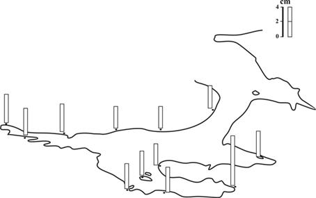
The greatest variations in the mean annual sea level take place in the estuaries of Onezhskiy and Dvinskiy Bays, the smallest ones occur in the northern part of the Bassein (the Chavanga station, Figure 4.27). Mean square deviations are 7.2, 5.4, and 3.0 cm, respectively. The range of interannual variations of the mean annual sea level reaches 37 cm in the rear part of the Onezhskiy Bay, 17-23 cm in Dvinskiy Bay, 17-22 cm in Kandalakshskiy Bay, 19 cm in the Gorlo, and 11-13 cm in the northern part of the Bassein (see Figure 4.27).
It is pointed out in Hydrometeorology and ... (1991), mean annual sea level variations exhibit a strong correlation at various points of Kandalakshskiy Bay. Mean annual sea level variations in Kandalakshskiy Bay, the Bassein, and Gorlo are also interrelated, which attests to the predominance of some general factors (e.g., water exchange between the White and Barents Seas) in the interannual sea level variations within these regions.
In the inner part of Dvinskiy and Onezhskiy Bays, the mean annual sea level variations have some specific features. The role of land runoff (mainly fed by the Severnaya Dvina River and Lake Onega) in the interannual sea level variability increases. Analogously, an increased role of land runoff fed by the Mezen and Kuloi Rivers can equally be expected for interannual level variations in Mezenskiy Bay.
It has been established by investigators of the Archangelsk Branch of Roshy- dromet in the late 1960s that the effect of atmospheric pressure upon the interannual level variations is significant and that its static component is predominant. At the same time, the influence of the wind is negligible. The effect of land runoff is limited to the estuaries of large rivers; it becomes insignificant at a considerable distance from the rivers.
These conclusions have been supported in further publications (e.g., Hydro- meteorology and .. ., 1991), which confirm that the river runoff accounts for about 9% of the dispersion of the interannual level variations in the Bassein and the estuary of Onezhskiy Bay, and for about 4% in the Gorlo and Voronka.
A certain portion of the interannual level variability arises from long-period tides. To estimate the lunar declination tide with an 18.6-year period, the method
|
(a)
(b)
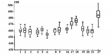
Figure 4.27. (a) The mean square of interannual variations of sea level (cm) in the White Sea and (b) fractiles of annual water level at the following stations: Kandalaksha - 1, Umba - 2, Kashkarantsy - 3, Chavanga - 4, Sosnovets - 5, Mudyug - 6, Severodvinsk - 8, Unsky Mayak
- 9, Zhizhgin - 16, Onega - 17, Raznavolok - 18, Kem Port - 19, Solovki - 20, Gridino - 21, and Kovda - 27.
described by Vorobyev (1969) has been employed. Inzhebeykin (2001) used in his calculations the mean annual sea level data for the 1950-1980 period for the White Sea. These data were collected at the Zhizhgin, Kovda, Kandalaksha, and Umba stations. In those locations the sea level regimes is only slightly influenced by the land runoff. The assessed phase and amplitude of the declination tide were further compared with the counter parameters of a static tide (Rossiter, 1967). The value of the declination tide (17.1 mm) was somewhat lower than that of the static one (18.6 mm), and the phase difference referenced to the year of 1950 constituted 73.6o. To estimate the sea level trend of the White Sea proper, we applied a preliminary smoothing technique to the initial time series by sliding the medians for five-year periods; the velocity value of the linear trend of the World Ocean level was assumed
to be an average of its estimated extreme values (i.e., +1.5mm year-1).
The results obtained have revealed that the level trends at various points have different signs and values: from -3.92 mm year-1at the Kovda station to
+1.04 mm year-1at the Unsky Mayak station. Taking into account the World Ocean level trend, a decrease in the White Sea level proper is observed at almost
every station. The values of linear trends presented in Table 4.4 show that mean annual sea levels at the stations located along the Karelskiy, Kandalakshskiy, and Terskiy coasts decrease from the Gridino station to the Kashkarantsy station with an average speed of about 3.0 mm year-1, and further on, up to the Sosnovets station, with an average speed of 2.0 mm year-1. At the same time, mean annual levels along the coasts of the entire Dvinskiy Bay become enhanced (if one neglects the linear trend of the World Ocean level). The only exception there is the mean annual sea level variation at the Severodvinsk station, where the data indicate a
Table 4.4. Linear trend of sea level variations at various stations in the White Sea, and the contribution of different mechanisms to the trend (mm year-1).
| Station | Period of observations | Trend of sea level (mm) | Coefficient of determination | Vertical movement of coast (mm year-1) |
| Kandalaksha | 1948-1985 | -2.12 | 0.759 | +3.62 ± 0.05 |
| Umba | 1934-1985 | -2.46 | 0.793 | +3.96 ± 0.05 |
| Kashkarantsy | 1954-1985 | -2.72 | 0.709 | +3.72 ± 0.05 |
| Chavanga | 1952-1985 | -1.22 | 0.528 | +2.22 ± 0.05 |
| Sosnovec | 1936-1985 | -1.51 | 0.429 | +2.51 ± 0.05 |
| Mudjug | 1937-1985 | +0.56 | 0.026 | -0.16 ± 0.05 |
| Severodvinsk | 1939-1985 | -0.62 | 0.195 | +1.12 ± 0.05 |
| Unsky Mayak | 1959-1985 | +1.04 | 0.170 | -0.54 ± 0.05 |
| Zhizhgin | 1939-1985 | -1.89 | 0.534 | +2.89 ± 0.05 |
| Onega | 1946-1985 | -1.64 | 0.320 | +5.54 ± 0.05 |
| Raznavolok | 1921-1985 | -1.6 | 0.635 | +4.3 ± 0.05 |
| Kem Port | 1920-1985 | -1.82 | 0.723 | +4.32 ± 0.05 |
| Solovki | 1924-1085 | -1.40 | 0.587 | +2.9 ± 0.05 |
| Gridino | 1947-1985 -2.25 0.824 +2.75 ± 0.05 | |||
| Kovda | 1947-1985 | -3.92 | 0.923 | +5.42 ± 0.05 |
|
sharp decrease in sea level. However, there are lacunes in the observations at this station. In addition, the available data were not always referenced to the adopted standard regarding the zero benchmark readings; hence an error may be expected. The largest absolute value of the sea level trend has been reported from the region of the Karelskiy coast (about -4 mm year-1, and taking account of the increased World Ocean level, nearly -5.5mm year-1).
These results partially differ from the simulated data. It can be due to a longer series of observations, and also to the fact that the simulated trends have not been verified for homogeneity over individual items.
The estimation of the contribution of various components to mono-directional level variations of the White Sea has revealed that it is the present-day tectonic motions of the sea s coasts that mainly contribute to such variations. Within the limits of the regions mentioned above, these motions result in both the elevation of the Karelskiy and Terskiy coasts with an approximately identical rate (about 4 mm year-1) and the sinking of the Zimniy and Letniy coasts with different rates.
Seasonal variability
On the whole, for seasonal variations of the White Sea level, characteristic are the presence of a major maximum in October and a major minimum in February (German and Pobedonostsev, 1977). There are some secondary local extremes but they are weak for the major part of the sea (except for the April minimum). The magnitude of seasonal sea level variations is different in various parts of the sea.
Based on the averaged long-term data, one can single out three types of annual sea level variation (see Figure 4.28). The first type is characteristic of a maximum in October and a minimum, most frequently, in February. According to the data from almost all sea level measurement stations located in the Bassein and Kandalakshskiy Bay, this area belongs to this type. Seasonal variations there are within the range 15-19 cm.
The second type has, apart from the major maximum in October, also a major minimum in February, two distinctly pronounced maxima in July and March, and two distinct minima in April and August. The value of the secondary minimum in April is close to, and at some locations lower than, the major annual minimum. The annual sea level variation is within 17-21 cm. This type is characteristic of sea level variations in the Gorlo, and Dvinskiy and Onezhskiy Bays.
The third and final type has two maxima and two minima occurring, respec- tively, in May and October and in August and March (Figure 4.29). This kind of variation in mean monthly sea levels takes place in the estuary zones of the Onega and Severnaya Dvina Rivers (and possibly other large rivers), where the value of the annual sea level variation (being averaged over many years) is maximal for the White Sea (23 and 80 cm, respectively).
The above-mentioned specific features of seasonal sea level variations in various regions of the White Sea are due to the following reasons: over the White Sea, winds of southern directions prevail during the period from December to March, whereas winds of northern directions are predominant in time interval extending from May
 (a)
(a)
(b)
(c)
Figure 4.28. Quantile diagrams of (a) maximal, (b) average, and (c) minimal seasonal vari- abilities of sea level (cm) at the Umba station (Point 2 in Figure 4.27).
to November. On the curves of the first type, the major minimum in February is due to both the transport of water from the White Sea by the prevailing south-westerly winds, most intensive in February, and also to the static effect of high atmospheric pressure over the White Sea in comparison with the Barents Sea (Figure 4.31). In October and November, the northerly winds are replaced by southerly winds; storms become more frequent there resulting in a wind-roughened surface, which is conducive to the major maximum in October.
Thus, it can be concluded that the monsoon regime (Dobrovolsky and Zalogin, 1982) is the predominant factor controlling the White Sea seasonal water level variations. The reported high coherence of variation in sea level and the assumed
|
 H (cm)
Q (%)
(a)
(b)
(c)
Figure 4.29. Fractal diagrams of (a) maximal, (b) average, and (c) minimal seasonal variabil- ities in sea level at the Onega station (Point 17 in Figure 4.27).
specific volume of water within the 0-50-m layer at the frequency corresponding to the annual period (German and Pobedonostsev, 1977), is only a consequence of predominance of the annual harmonic amplitude in both cases. That is why German and Pobedonostsev (1977) failed to reveal a phase shift of 1.4 months in the annual variations of the conditional density and sea level. The increased water density, mainly caused by the water temperature decrease and partially by a higher compensatory income of more saline waters from the Barents Sea as well as by a decrease in the land runoff, only accentuate the sea level minimum occurring in February.
The second type of annual sea level variations, with more pronounced secondary extremes, is observed in the regions where the influence of both the land runoff, and the resulting water exchange with the Barents Sea, is stronger. Such regions are: Dvinskiya and Onezhskiy Bays, the Gorlo, and apparently the Mezen Strait and the Voronka. A secondary maximum occurring in June-July is a consequence of super- position of storm-driven surges caused by northern winds that are very high at this time of year, and spring river floods. The secondary minima in April (which are often more pronounced than the major minimum in February) and August are due to the insignificant river runoff during the phase of, respectively, winter and summer low- water flow. A weak peak in March is possibly due to the increased share of waters flowing from the Barents Sea (Inzhebeykin, 1981) in the net water exchange between these two seas. Because of the climatologically moderate area of the region under investigation, any other factors (atmospheric pressure, evaporation from the water surface, precipitation, water density variations) cannot produce the difference in seasonal sea level variations in the north-western and south-eastern regions of the White Sea, since the absolute values of the relevant factors in these areas are nearly equal, and their variations throughout a year approximately identical. However, the contribution of seasonal variations of precipitation to the variability of sea level on the same scale is rather considerable and can constitute (Hydrometeorology and .. ., 1991) up to 3.8 cm (18-25% of the seasonal sea level variations) with a minimum in February-March and a maximum in August-September.
For sea level variations, the absolute magnitudes of precipitation and evapora- tion are not as essential as their difference, which characterizes the air moisture just above the water surface. Generally, seasonal variations of precipitation and evapora- tion are not synchronous. Therefore, the seasonal distribution of this parameter averaged over the entire sea has maxima in January (35mm) and July (7.4 mm), and minima in April (5.7 mm) and October (5.9 mm) (Hydrometeorology and .. ., 1991). Thus, the contribution of the algebraic sum of precipitation and evaporation to the seasonal sea level variations constitutes 2.9 cm, and the minimum sea levels in April, observed in the annual level variations of the second type, are in part due to this factor.
The estimation of contributions of atmospheric impacts to level variations, performed for the Kem-Port and Sosnovets stations (located in different regions of the sea) has revealed that the static and wind response of the sea level to atmo- spheric pressure variations accounts for 10 to 50% and 30% of the total dispersion, respectively (Hydrometeorology and .. ., 1991).
|
However, the local atmospheric pressure, having in the autumn-winter period a higher magnitude than that over the entire Barents Sea, reflects indirectly the pre- valence of the south-western transport in wintertime. Thus, the results reported in Hydrometeorology and ... (1991) are essentially consistent with our conclusion that the monsoon regime is the principal player controlling the seasonal water level variations over the major part of the White Sea.
The influence of river runoff upon the seasonal variations of sea level of the third type for the stations located in estuaries of large rivers is obvious. The maxima in May and October are due to spring and autumn floods, and the minima in April and August are the consequence of very low river runoff during the winter and summer mean water phases (Figure 4.33). As mentioned above, the maximal seasonal water level variability occurs exactly in these regions of the White Sea.
The pole tide
A forced wave, which is formed in the world s oceans due to the Earth s centrifugal force variations (that are relevant to displacements of the instantaneous axis of the Earth s rotation), has been coined the pole tide by G. Darwin (see Maksimov, 1970a). The Earth s centrifugal force changes as a result of the 14-months free and 12-months forced oscillations of the Earth s rotation axis or motions of the instan- taneous pole of the Earth s rotation (Maksimov, 1970b). The pole tide , with a period close to 14 months, is a standing wave with antinodes at 45oN and 45oS and nodes at the poles and the equator. In the White Sea (located between 63oN and 69oN) the pole tide is highly pronounced (Inzhebeykin, 2001).
To evaluate the pole tide , the so-called method of separating tables suggested by G. Darwin has been used (Maksimov, 1970a, b). The method consists of the following. Mean monthly sea level variations are arranged as separate 14-month series and are averaged over the time intervals of 7, 14, 21, 28, ... years. Given this way of averaging, the 12-month sea level variations also participate in the averaging procedure but with inverse (opposite) phases and, hence, are completely excluded. Therefore, the remaining variability accounts exclusively for the 14-month variations. The ordinates obtained in this way have been subjected to a harmonic analysis, and the amplitudes and phases averaged over a 7-year period have been quantified (Maksimov, 1970a). To obtain more precise results, 7-year periods were shifted, one relative to another, by three years. The calculations were conducted for the periods 1950-1956, 1953-1959, etc., for the Sosnovets, Zhizhgin, Solovki, and Kem-Port stations, where the effect of river runoff on sea level varia- tions was insignificant (Figure 4.30).
The results of calculations have revealed that the amplitude of the pole tide varies between 1.2 and 4.3 cm nearly synchronously at all four stations with a period of 18 years (Figure 4.31). The pole tide phases obtained for individual stations confirm the theoretical assumption that this tidal wave propagates from the west eastwards. For instance, for the Zhizhgin station, an average co-tidal month (the time interval between the moment of the passage of the instantaneous pole of the Earth s rotation through the Greenwich meridian and the formation of the pole tide
 |
 Figure 4.30. Variations of sea level as assessed by the Darwin method at the following stations: Sosnovets (1), Zhizhgin (2), Solovki (3), and Kem Port (4).
wave maximum) constituted 12.8 months, whereas for the Sosnovets station it exceeded 12.9 months. Averaged over the four stations, the co-tidal month of the pole tide wave for 1950-1980 appeared to be 12.9 months. The data obtained for the pole tide confirm the results reported by Maksimov (1970b), according to which the tidal amplitude varied with a period close to 18 years, and the co-tidal month was equal to 13.4 months.
The pole movement, along with the 14-month variations, exhibits oscillations with a 6-7-year period, which are due to a superposition of free variations with a period of 14 months and forced ones with a period of 12 months (Karklin, 1967). Obviously, the pole movement variations with a period of 6-7 years can cause pole tide variations with the same period.
4.7.2 Synoptic variability
The variability of the White Sea level in the synoptic frequency range is rather significant and nearly equals the tide-driven variability. Statistical processing of hourly sea level non-periodic constituents during some given (mostly annual) periods has shown that the greatest amplitude of non-periodic variations (see Figure 4.31) occurred in the inner parts of the Onezhskiy and Mezenskiy Bays (3.55 and 2.81 m, respectively), whereas the smallest one is typical of the Bassein and Kandalakshskiy Bay (about 1.3 m).
The root mean square deviation of these variations from the mean sea level
|
 (a)
(a)
(b)
Figure 4.31. (a) Amplitude and (b) root mean square deviations of the White Sea mean level.
(considering only a year-long series) displays its maximum in the Onega Bay (35.5 cm) and its minimum in Kandalakshskiy Bay (about 17 cm) (Figure 4.31). Practically for all stations, the distribution of ordinates of non-periodic variations exhibited both a positive asymmetry and excess (i.e., it departs from the normal distribution (Figure 4.32)). In terms of the absolute magnitude, positive deviations

Figure 4.32. Storm surge distribution (%) in (a) Dvinskiy Bay and (b) across the remaining part of the White Sea.
from the mean sea level are usually much greater than negative ones (i.e., the number/density of surges exceeds that of sea level decreases).
The greatest recurrence of storm-driven surges in the White Sea is observed in September-December, when the cyclonic atmospheric activity over the White and Barents Seas significantly increases (Figure 4.32). In winter, the ice cover restrains an appreciable sea level increase. In summer the atmospheric cyclonic activity is negligibly low.
The relationship between non-periodic sea level variations t;(t) and the driving forces can be described precisely enough as a process at the exit of a linear dynamic system with two processes and two constant parameters as inputs. One of the param- eters is the wind speed projection (t) upon the effective positive-negative surge direction (when maximal non-periodic sea level variations take place). The other parameter is the surface atmospheric pressure p(t) (German, 1975; Glukhovskikh et al., 1975; German and Levikov, 1979). A strong aspect of this approach, outlined in detail by Bendat and Piersol (1974), is the possibility of preserving the frequency structure of signals, as well as the possibility of evaluating the relationship between sea level variations and the relevant external factors (e.g., wind and atmospheric pressure) even for the options corresponding to a zero influence of any of them.
The obtained spectra of non-periodic sea level variations during May- November, 1966 are indicative of having a period of 4 to 5 days (Figure 4.33). However, the relevant energy spectra display only a slightly pronounced correspond- ing maximum, whereas a maximum at the frequency of 1/210 cycles per hour (about 8-9 days) is distinctly expressed (Figure 4.33).
It has been found from multiple and partial coherence functions that in the frequency range f = 1/105 - 1/210, for all cases under consideration, there exists a close relation between the meteorological elements and sea level variations. For instance, for the Kem-Port station, at f = 1/105 cycles per hour, the value of the multiple coherence function is 0.83, and the partial coherence functions are equal to
0.77 and 0.70, respectively.
|
 |
 Figure 4.33. Frequency spectrum of sea level variations at the Kem Port (1) and Mudyug (2) stations.
On the whole, such an agreement confirms the above conclusion regarding storm-driven surges in the White Sea owing to displacing cyclones, which move over the White and Barents Seas mostly from the west eastwards with a periodicity of 4-6 days. A close linear relationship between non-periodic sea level variations and the effective wind constituent and atmospheric pressure accounts for the agreement between the observed and retrieved spectra in the above frequency range. It has been found that for the Kem-Port and Onega stations, the effective direction is 0o, whereas for the Archangel and Mudyug stations it is 335o, and 225o, respectively. At stations located nearby Archangelsk and in Onezhskiy Bay, the main peak in the spectral distribution of sea level variation density is observed at lower frequen- cies, corresponding to a period of 17-20 days. On the other hand, for periods of such duration, the values of multiple and partial coherence functions are small. The revealed displacement to the low-frequency region of spectral maxima of sea level variations in the estuaries of the Severnaya Dvina and Onega Rivers may apparently
be accounted for by the effect of river runoff.
For nearly all points in the low-frequency region (9-30 days), the variations of sea level and atmospheric pressure are opposite in phase (120-170o), which points to the dominating role of the well-known reverse barometer effect at these frequen- cies. This is in accordance with the conclusions of other workers experimenting elsewhere and stating that the static reaction is characteristic of a range of periods from a few dozen to several hundred hours. At higher frequencies (up to a 3-6-day
period), the phase shift is negligible (from 0o at the Kem-Port station to 57-60o at the Archangelsk and Onega stations). This is indicative of an enhanced role of dynamic factors at these frequencies.
The actual role of a concrete factor in generation of storm surges depends on the cyclone type. In synoptic meteorology the most common classification of cyclones is that relevant to the trajectories of their movement. Potanin (1972) suggested this typification of cyclones specifically for the investigation of surges in the Barents and White Seas. Proceeding from the analysis of cyclonic movements during the period 1902-1965, he classifies the moving cyclones into diving , western, southern, and abnormally displacing ones. Inzhebeykin (2001) shows that with western cyclones, the mechanism of formation of storm-driven surges owing to cyclones can be different and is dependent on whether the cyclone center passes over the Barents or White Seas (or to the south of the latter). Therefore, while Potanin (1972) considers western cyclones in general, Inzhebeykin subdivides them into the
Barents Sea western and White Sea western ones.
The recurrence rate of cyclones of the diving and western types is about 88%. Thus, surges in the White Sea are mainly caused by the arrival of deep cyclones of the first two types, which is due to the cyclogenesis processes taking place at the Arctic ( diving cyclones) and polar (western cyclones) climatic fronts (Figure 4.34).
The surge that occurred on 2 November, 1963 is a typical example of the phenomenon driven by diving cyclones. The cyclone that caused the surge in question was moving south-eastward at a speed of 40-50 km h-1along an upper- level frontal zone. By the onset of the sea level elevation at the Archangelsk station, the cyclone was moving over the Barents Sea (Figure 4.34(a)). The atmospheric pressure in the centre of the cyclone was about 990 HPa. The conditions for cyclone deepening were quite favorable because it was a temperature-asymmetric cyclone, in which warm and cold sectors were distinctly expressed. The atmospheric pressure drop at the sea surface constituted 6.5HPa over 3 hours, and its rise equaled
4.7 HPa over 3 hr. In the Barents Sea a long wave was formed, which propagated from north-west to south-east and further on to the White Sea. The wave trough reached the Sosnovets station at approximately midnight, 1 November, and the Archangelsk station at 0900, on 1 November. The wave crest reached the Sosnovets and Archangelsk stations at 1100 and 1800, 2 November, respectively. Thus, the wave propagation speed was higher for the wave crest than for its trough. At the moment of maximum surge in Archangelsk, the cyclone centre displaced in the north-easterly direction.
Date: 2016-03-03; view: 698
| <== previous page | | | next page ==> |
| Oceanographic regime 4 page | | | Oceanographic regime 6 page |