Oceanographic regime 4 page

The experiments conducted in the estuary of the Onega River have revealed some essentially non-linear effects in tidal currents and sea level fluctuations, the latter being expressed in the time difference between the level decrease and increase. The main cause of these non-linearities proved to be the bottom friction effect. Besides, the difference between the mean sea level and high-water level was

Figure 4.17. Frequency spectra of sea level and water surface temperature variability in Kandalakshskiy Bay.

somewhat larger than that between the mean sea level and low-water level, which indicates the presence of a residual tidal circulation in the White Sea.

Temporal distributions of current speed and direction are more complicated and do not comply with a purely harmonic type. It is particularly well pronounced during the syzygy tide, given a medium or minimum river discharge rate. Calculated char- acteristic speeds of tidal movements for the mouth of the Keret River are in fair agreement with the observed values.

A similar pattern of water temperature and salinity distributions was recorded in September in Onezhskiy Bay. A characteristic pattern of vertical distribution of water temperature and salinity in the deep-water part of the Bay in July and September is exemplified in Figure 4.10. As seen, water mixing over the entire water column is observed at all stations in September. In shallow areas, the mixing is most pronounced in July, when weak water stratification is observed. This may be due to strong tidal currents flowing in the bay coupled with autumnal water cooling.

Figure 4.18. Variability of current speed and direction in the estuary of the Kem River at an 8-m depth (4-7 July, 2000).

The existence of water temperature variability in conditions of water column stratification indicates the presence of internal wave fluctuations with a period of semi-diurnal tidal motions (Figure 4.19, see color section). The intra-wave fluctua- tions have the largest amplitude at depths between 11 m and 21 m, and they are greatest in the upper layers (within the layer of a 4-8-m thickness). The presence of small-scale variations may point to an instability of intra-wave fluctuations, given there is a speed shear in the near-bottom layer.

Water temperature observations accomplished in the region of the Kuzovskie Islands employing the TR-2 temperature profile recorder at depths of 10 m (Figure 4.19, see color section), make it possible to conclude that there is a close relationship between water temperature variability and the tidal phenomena. The water tempera- ture difference between the surface and 10-m depth did not exceed 0.5-1.0oC.

The water temperature variations displayed in Figure 4.19 (see color section) also correspond to the semi-diurnal tidal pattern. The time coincidence between the appearance of high and low-tide extremes and speed maxima indicate the progressive nature of the tidal wave.

As discussed above, a residual tidal circulation is inherent in the White Sea. This phenomenon is highly consequential in terms of pollutant propagation across the White Sea: the impurities, once entrained by the river runoff and tidal currents, continue their migration under the influence of residual tidal motion (this process being irreversible).

4.6 MODEL STUDY OF CURRENTS AND MASS TRANSPORT PROCESSES IN SOME BAYS AND ESTUARIES

The issue of transformation of the tidal wave and transport of admixtures in shallow-water bays and estuaries was thoroughly discussed in Russian publications

(see e.g., Lupachev, 1989; Zyryanov, 1995). The estuary of the Severnaya Dvina River has thus far been studied most comprehensively. The process of propagation of pollutants in the tide-affected estuary of the Severnaya Dvina River was investi- gated by Brekhovskikh et al. (1997), who used a mathematical model to simulate the propagation of pollutants under the normal regime of functioning of water treatment installations of pulp-and-paper mills as well as for the case of an emergent water release. Potential ecological consequences of emergent water release were estimated. It has been shown that the combination of a tidal current in the Severnaya Dvina River and transverse advective transport in the zone of the dispersed plume may result, under certain conditions, in pollution of a city water intake facility during the winter dry-weather period. Brekhovskikh et al. (1997) developed a 2-D mathematical model for simulating the propagation of passive admixtures with the sub-ice tidal flow. The model has been verified employing in situ data from the estuary of the Severnaya Dvina River. It is shown that in the presence of ice cover, and in con- ditions of low water discharge into the estuary of the Severnaya Dvina River, a more intensive water mixing and expansion of the stream of pollutants in the opposite direction occurs.

As objects for investigation, shallow-water coastal areas of the estuaries of the Onega and Kem Rivers were chosen, as well as the region of the estuary of the Keret (Srednyaya Salma) River, Nikolskiy Bay, and entire Onezhskiy Bay (Figure 4.20). For all these marine regions, numerical simulations of the tidal circulation were performed for different sets of conditions and different patterns of transport of a conservative admixture. This was achieved making use of detailed coordinate grids. The validity of the results thus obtained has been further confirmed by a thorough comparison with the available in situ data.

4.6.1 A brief description of the model for simulating estuarine currents

For numerical simulations, the hydrodynamic modeling system CARDINAL (Coastal Area Dynamics INvestigation ALgorithm) (Volzinger and Piaskovsky, 1977; Ramming and Kowalik, 1980; Klevanny and Matveyev, 1994) has been used. The model encompasses a system of equations for a shallow-water case, taking into account the horizontal transport and turbulent diffusion in curvilinear coordinates. The model is intended for studying coastal water dynamics. The use of a curvilinear coordinate system is particularly convenient for modeling coastal zones that include bays, estuaries, islands, and peninsulas. The dynamic equations are solved using a semi-implicit finite-difference method, which makes it possible to use relatively large time increments.

The shallow-water equations take the form:

dw dw dw

dt + A dx + B dy = F

u

u 0 g

0 0

w =

A = 0 u 0

B = 0 g

h

H 0 u

0 H

Figure 4.20. Bays and estuaries (denoted by circles) in the White Sea Basin used for modeling

and verification experiments.

Dxdh

l + H + aAu + g dx

F = Dy

where (u, ) are the constituents of the current speed vector, H = h + z is the depth, z

is the sea level, g is the gravitational acceleration constant, l is the Coriolis

parameter, Dx and Dyare vector components of the tangent stress of the wind, and a

is the coefficient of horizontal turbulent exchange.

The equation of transfer and diffusion of a non-conservative admixture takes the form:

dC dt +

d( uC)

dx +

d( uC)

dy =

d( kdC/ dx)

dx +

d(kdC/ dy)

dy + I - rC

where k is the coefficient of diffusion, I is the source function, r is the coefficient of non-conservativeness, and C is the admixture concentration.

This model makes it possible to perform calculations of currents, water-level fluctuations, and concentrations of pollutants in a water body.

The CARDINAL modeling system makes it possible to address a wide range of hydrodynamic and ecological problems, such as to:

• Determine the future influence of human activities (such as planned hydrotech- nical constructions, such as dams, water treatment installations, wavebreaks, and sand pits in rivers, pens and ponds) upon the hydrodynamic regime and pollution rates of aquatic areas, as well as to suggest their optimal location.

• Work out recommendations on improvement of a water basin s ecology.

• Elaborate precautionary measures for elimination of the consequences of acci- dental pollution of water bodies.

• Create a system of integrated sustainable management of regional water resources that, in particular, provide for the design of optimal plans for the development of the infrastructure of objects relevant to the aquatic environment.

• Perform calculations and online forecasts of water level variations during marine inundations.

• Perform a classification of various localities in the coastal zone, depending on the extent of danger from storm waves.

4.6.2 Onezhskiy Bay

Onezhskiy Bay is one of the largest bays in the White Sea. It is also the shallowest. It is oriented from north-west to south-east. Its area is 10,000 km2, its length is 185km and its mean depth is 17 m (with its greatest depth being 80 m). The water volume of the bay is 160 km3. The bottom relief is rather uneven, especially along the bay s western coast, where there is a great number of islands (Figure 4.21).

Onezhskiy Bay is linked with the central part of the Sea by two straits, namely, the western and the eastern Solovetskiy Salmas Straits. The rather deep-water Salma Straits provide access for great amounts of water to enter the bay. Since the entire bay is shallow, strong tidal currents arise. The largest tributaries are the Onega, Kem, and Vyg Rivers. The maximum speed of a syzygial tide is 1.5-2.0 m s-1in the eastern Salma Strait, and 1.5-1.7 m s-1in the western Salma Strait. The tidal currents in the Solovetskiy Salmas Straits are bidirectional by nature. In the open part of the bay, the current speeds amount to 1.0 m s-1, and in the estuary of the Onega River they are 1.4-1.5m s-1. A superposition of wind and tide-driven currents

Figure 4.21. Bathymetry of Onezhskiy Bay and location of sea level tide gauges (denoted by dots).

can increase the speeds of the resultant currents up to 2.0-2.5m s-1(Lifschitz, 1984). However, wind and gravity-driven currents, due to the wind field variability over the bay and low river discharge rates, cannot significantly affect the formation of resultant currents.

To account for the highly irregular coastline of the bay, the presence of islands therein, as well as some specific features of the bottom relief, a curvilinear coordinate grid has been drawn with a space step of 2-3 km for the entire Onezhskiy Bay, and about 1 km for the estuary region of the Onega River.

At the northern boundary of the White Sea, the amplitude and period of tide- driven variations in sea level were set at 60 cm and 12 hr 25min (the M2 wave) (Hydrometeorology .. ., 1993). The friction coefficient was assumed to be 0.014. The advective terms in the equations of motion were ruled out, and the Onega River discharge was neglected.

At the apex of the bay, the moments of high and low water correspond to minimal current speeds of the order of 12 cm s-1, whereas the moments of a zero- level position are characterized by maximal current speeds of about 75-100 cm s-1 (a standing wave). In the middle part of the water area, current speeds vary within the

range 40-60 cm s-1at the moments of high and low water, and within the range 6- 85cm s-1at the moments of an equilibrium level position (the forward-moving- standing wave type). In the vicinity of the boundary, maximal speeds correspond to the moments of high and low water and reach 75-100 cm s-1. At the moments of zero-level positions, the speeds are minimal and of the order of 10-40 cm s-1(a forward-moving wave). Maximal current speeds are observed in the straits in the area of the Solovetskiy Archipelago and Kondostrov Island, and can be as high as 150-200 cm s-1. Thus, across the major part of Onezhskiy Bay, a mixed (forward- moving-standing) wave type prevails (Figure 4.22).

The data on sea level variations from tide gauges are presented in Figure 4.23. At the outer part of the bay, the amplitude of water level variation is 60 cm. As one moves deeper into the bay, the amplitude of water level variation at first decreases to 40-50 cm, and later increases up to 80 cm in the middle part of the bay, and even up to 110 cm at the bay s apex. At the entrance to the bay, the period of water level growth (6 hr 10 min) nearly equals that of the water level decline (6 hr 15min). In the middle part of the bay, the level growth period is, on average, 1 hr 30 min less than that of the water level decline. In shallow-water coastal areas, a clearly pronounced non-linearity of the water level variation is observed: the level growth period is much less than that of water level decline (by 4-5hr). In the coastal zone, the level inequal- ity between high and low water phases is observed. It reaches 60 cm (mareograph no. 8). Mareograph no. 4 data reveals that the water level growth period is 6 hr 20 min, which is greater than that of the decline (6 hr 5min).

4.6.3 Estuary of the Kem River

Tidal oscillations of the water level in the White Sea originate at the entrance to the Solovetskiy Salma Sraits a forward-moving tidal wave that propagates toward the inner part of the Onezhskiy Bay. In the outer part of Onezhskiy Bay, the tidal wave is mainly forward-moving and has an amplitude of about 60 cm, the maximum speed of the tidal current being as high as 150 cm s-1. Obviously, the tidal variations of the sea level in the estuary of the Kem River must be controlled by the specific features inherent in the tides propagating in the estuary zone.

To take into account the highly irregular shape of the coastline in the estuary area as well as the presence of islands and the specific features of the bottom relief, a curvilinear coordinate grid with a spatial step of 100-250 m was employed.

At the boundary of the area, tidal oscillations were assumed to have an amplitude of 65cm and a period of 12 hr 25min (the M2 wave). The calculated spatial distributions of tidal current speeds and sea level for a single tidal cycle are illustrated in Figure 4.24.

During the high-tide phase (50 hr 00 min), the current speeds are insignificant. Throughout the major part of the water area they constitute 5-25 cm s-1. In between the islands and in the estuary of the Kem River, they increase up to 35cm s-1. During the low-tide phase (56 hr 10 min), the current speeds do not exceed 20 cm s-1 across the major part of the water area. In the strait between the

Figure 4.22. Calculated current speed and sea level distributions across Onezhskiy Bay (numerical calculations for a 30-hour and 40-hour period during the low-water phase at the bay s apex).

120 5

60 8

-20

-40

-60

-80

-100

27 30 33 36 39 42 45 48 Hours

-120

Mareograph 1

Mareograph 3

Mareograph 5

Mareograph 8

Mareograph 9

Figure 4.23. Water level variations as obtained from tide-gauge measurements (station nos. 1, 3, 5, 8, and 9, see Figure 4.21).

continent and Yakostrov Island, the current speeds increase to 30 cm s-1. In the estuary of the Kem River the current speed can be as high as to 40 cm s-1.

Throughout the phase of low water (59 hr 15 min), the current speeds increase to 50-100 cm s-1, in the narrows they become as high as 50-200 cm s-1. The discharge current from the estuary of the Kem River is very well developed in this phase of the tidal cycle: its speed reaches 75cm s-1.

Therefore, the periods of high and low water correspond to maximal current speeds, whereas minimal speeds pertain to the periods of high and low tide, which means that, for a given water area, the forward-moving type of the tidal wave is characteristic.

4.6.4 Turbulent diffusion of a conservative pollutant in the coastal zone of the Onezhskiy Bay and the Kem River

The main source of pollution in the Onezhskiy Bay is discharge waters incoming with river runoff, whose average annual volume is 45km3. This amounts to about 20% of the volume of the total freshwater discharge into the White Sea. The biggest

(a)

(b)

Figure 4.24. Calculated spatial distributions of current speeds and water levels for a single tidal cycle. High-water (a; 5hr 00 min) and low-water (b; 59 hr 15 min) phases in the estuary of the Kem River.

tributaries of the bay are the Onega, Kem, and Vyg Rivers (with annual discharge rates 18.0, 8.3, and 7.8 km3respectively). There are fish farms in the estuaries of these rivers. The hydroelectric power station cascades have been built on the rivers (Kem, Vyg, Kovda, and Niva) flowing into the Onezhskiy and Kandalakshskiy Bays. A negative impact of these hydroelectric power station cascades on the natural environ- ment becomes highly apparent through flooding of lands, alterations in fish popula- tions and species composition, as well as in deterioration of water quality. The dams of hydroelectric power stations hinder fish migration and their movement toward spawning areas as well as the descent of young fish from head river waters to marine water. The hydroelectric power station cascades on the Kovda, Vyg, and Kem Rivers significantly reduced the populations of the most valuable species, such as salmon and white-fish.

Before the hydroelectric power station on the Niva River was constructed, the river was a well-known spawning area for salmon; after the hydroelectric power station was erected, the pathways for the fish were locked, and the spawning area ceased to exist (Sidorenko and Mitrukova, 1994).

In the upstream area of the Kem River, the Kostomuksha ore mining and processing enterprise was put into operation in 1984. The effluents from this enter- prise, brought with the Kem River, began entering the Yushkozero water storage reservoir (Sabylina, 1983).

The main sources of pollution of the Vyg River are hydroelectric power stations, ship cruising along the route of the Belomorsko-Baltiysky Canal, timber rafting, fish-farming/processing, and forest melioration. The sewage waters of the Segezh pulp-and-paper mill (put into operation in 1939) and the Nadvoitsk aluminium plant (operating from 1954) flow into the Vygozero water storage reservoir (Lozovik et al., 1989). The Onega River is a source of water supply for both the local population and the enterprises. In addition, this water way is used for timber rafting, as a water transport route, and also as a collector of sewage water (Sabylina, 1983). The pulp-and-paper production and industrial hydrolysis works are extremely water-consuming.

Making use of numerical modeling, the transport of conservative admixtures/ pollutants was studied. The pollutants are brought to Onezhskiy Bay with the waters discharging from the Onega River by tidal and gravity currents. The modeling of specific features of the tide-driven transport of water and pollutants was performed with the help of the CARDINAL program. To take into account the jagged shape of the coastline, the presence of islands, and specific features of the bottom relief, a curvilinear coordinate grid with a space step of 2-3 km was applied for the entire Onezhskiy Bay; grids with a space step of about 1 km were employed for the estuary region of the Onega River, and a grid with a 50-150-m step for the estuary of the Kem River.

All model calculations were performed for a maximum possible number of nodes of the gridded area to reproduce most reliably the morphometric features of the area under consideration. At the entrance to the Onezhskiy Bay, a semi-diurnal wave with a 60-cm amplitude was set. Figure 4.25 presents the pollution plume dispersion in the estuary region of the above rivers 72 hr after the model was

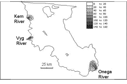Figure 4.25. Areas of propagation of pollution in Onezhskiy Bay (72 hours after the model initiation).

initiated. The farthest distance (20 km) of the polluted matter transport from the source (river outfall) was found in Onezhskiy Bay. The pollution dispersion proceeded along the right-hand coast of the bay in accordance with the existing scheme of permanent currents. In the regions neighboring the estuary of the Kem and Vyg Rivers, the pollution plume extended over 15 and 12 km, respectively, over the period of calculations.

Estuary of the Kem River

To investigate the propagation patterns of conservative admixtures in the estuary of the Kem River, two experiments were conducted. The first experiment consisted of obtaining the pattern of admixture transport across the water area during a single tidal cycle. The second experiment was the study of impurity transport during 3 tidal cycles for different river discharge rates. The calculation was performed for three options of river discharge rate: in the first case, the river discharge was assumed to be 97 m3s-1, which corresponds to a minimum discharge level for the given river; in the second case, the discharge rate was assumed to be 260 m3s-1, which is the annual average discharge for the Kem River; finally in the third case, the discharge rate was taken to be 500 m3s-1, which is characteristic of the spring tide in the Kem River. In the first experiment, in order to monitor the transport of admixtures by tidal currents throughout the water area of the estuary of the Kem River, the admixture propagation was calculated per single tidal cycle, with an interval of 1 hr, starting with the moment corresponding to 74 hr after the model initiation. The simulations

were carried out for the mean annual river discharge rate.

The following specific features of the tidal transport of admixtures throughout the water area have been revealed. At the moment of equilibrium position of sea level during the high-tide phase (74 hr 40 min), the plume extends along the coast as a narrow strip. The impurity concentration is maximal in the middle part of the strip, 2 km off the source. Then the plume pattern changes radically. At 75hr 40 min, the plume at the exit of the estuary of the Kem River begins to displace to the right. At the moment of high water (77 hr 40 min), the main admixture stream is located to the south of Yakostrov Island. There the maximal impurity concentrations occur along the coastline. At the moment of equilibrium position of the water level during the low-tide phase (80 hr 40 min), the tidal stream transports the entire plume to the right and southward with respect to the estuary of the Kem River. During the next three hours of low tide, the impurity stream quickly returns to its former position. By the moment of the low-water phase (83 hr 40 min), the plume spreads over the entire space between the coast and Yakostrov Island. Low admixture concentrations are observed at the lakeside of the island; during the next two hours the plume is drawn by the current to beyond the limits of the grid region. With the onset of high tide (85hr 40 min), the plume again extends along the coast acquiring the form of a narrow strip. Figure 4.26 shows the position of plume during three tidal cycles after the model initiation for minimal (a) and maximal (b) options of the discharge rate of the Kem River.

For a minimal discharge rate, the plume remains rather sedentary and the densest part of it fails to escape from the estuary during the computation time. In the case of a medium or maximal discharge rate, the plume moves upwards from the estuary for a distance of 3 or 4 km, respectively. The distance of admixture propaga- tion off the estuary to the right is 1.5km for the minimal discharge rate and 2 km for the medium or maximal discharge rate options. The width of the densest plume for the cases of minimal, medium, and maximal discharge rate options is 100, 250, and 500 m, respectively.

The simulated values of currents and level oscillations in some bays and estuaries of the White Sea were compared with the relevant in situ measurements. The obtained modeling results regarding the specific features of water circulation and conservative impurity propagation in different phases of the tidal cycle, within the estuaries of several rivers discharging into the White Sea, constitute a basis for the estimation of potential propagation of sewage waters, assessing the consequences of emergency discharge, and for undertaking the necessary measures to assure ecolo- gical safety of the sea.

4.7 SEA LEVEL VARIATIONS AND TIDES

This section expands upon the issue of sea level fluctuation in the White Sea. The fluctuations are assessed within a wide range of time scales. The prevailing contribu- tion of semi-diurnal and diurnal tidal movements into the variance spectrum is substantiated. Importantly, the tide of the White Sea proper proves to be far lower than the induced tide originating in the Barents Sea.

(a)

(b)

Figure 4.26. Location of the plume three tidal cycles after model initiation for (a) minimal and

(b) maximal options of the rate of discharge of the Kem River.

4.7.1 Large-scale sea level fluctuations

Large-scale water level fluctuations in the White Sea, which have timescales ranging from several months to hundreds of years and which occur across the entire sea, are formed under the influence of atmospheric processes, river runoff, evaporation, precipitation, and water density variations (having a strongly pronounced seasonal nature), as well as water exchange with the Barents Sea and the vertical motions of the earth s crust. On these scales, given the scope of observations in the White Sea, the most essential variations are seasonal, interannual, and intra-secular. Consider in more detail their respective contributions to long-term fluctuations of sea level in the White Sea.

Date: 2016-03-03; view: 571