CATEGORIES:
BiologyChemistryConstructionCultureEcologyEconomyElectronicsFinanceGeographyHistoryInformaticsLawMathematicsMechanicsMedicineOtherPedagogyPhilosophyPhysicsPolicyPsychologySociologySportTourism
Average, Marginal and Total Product. Law of diminishing returns
In the short run, the relationship between the physical inputs and output can be describes from several perspectives.
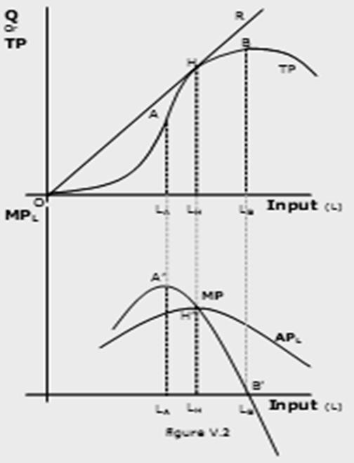 Total product (TP or Q) is the total output. Q or TP = f(L) given a fixed size of plant and technology. Average product (APL) is the output per unit of input. AP = TP/L (in this case the output per worker). APL is the average product of labour. Marginal product(MPL) is the change in output "caused" by a change in the variable input (L), so MPL = ∆Q/∆L.Over the range of inputs there are four possible relationships between Q and L
1) TP(Q) can increase at an increasing rate. MP will increase (from O to LA.)
2) TP in inflection point- MP max. TP may increase at a constant rate-MP will remain constant in this range.
3) TP might increase at a decreasing rate- MP fall.(from LA to LB)
4) If "too many" units of the variable input are added to the fixed input, TP can decrease, in which case MP will be negative.
The average product (AP) is related to both the TP and MP. At LH level of input, APL is a maximum and is equal to the MPL. When the MP is greater than the AP, MP "pulls" AP up. When MP is less than AP, it "pulls" AP down. MP will always intersect the AP at the maximum of the AP.
Law of diminishing returns means that as the level of a variable input rises in a production process in which other inputs are fixed, output ultimately increases by progressively smaller increments. The law of diminishing marginal product says that if we keep increasing the employment of an input, with other inputs fixed, eventually a point will be reached after which the resulting addition to output (i.e., marginal product of that input) will start falling.
A somewhat related concept with the law of diminishing marginal product is the law of variable proportions. It says that the marginal product of a factor input initially rises with its employment level. But after reaching a certain level of employment, it starts falling.
The reason behind the law of diminishing returns or the law of variable proportion is the following. As we hold one factor input fixed and keep increasing the other, the factor proportions change. Initially, as we increase the amount of the variable input, the factor proportions become more and more suitable for the production and marginal product increases. But after a certain level of employment, the production process becomes too crowded with the variable input and the factor proportions become less and less suitable for the production.
37. Producer’s behavior
Producers try to maximize profit, provides the motivation for their behavior. They must make plans while confronting uncertainty about:
-Consumer demand, -Resource availability, -Intentions of other firms in the, -Industry. For making decision producers use isoquant and isocost.
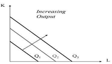
Isoquant is just an alternative way of representing the production function. Consider a production function with two inputs factor 1 and factor 2. An isoquant is the set of all possible combinations of the two inputs that yield the same maximum possible level of output. Each isoquant represents a particular level of output and is labelled with that amount of output.
Isocost line– a line that represents alternative combinations of factors of production that have the same costs. Or in other words, the combinations of inputs (K, L) that yield the producer the same level of output.
Cost minimization (Producer’s choice optimisation)
The least cost combination of inputs for a given output occurs where the isocost curve is tangent to the isoquant curve for that output.
The slopes of the two curves are equal at that point of tangency.
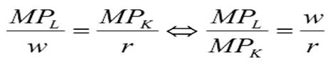
The firm is operating efficiently when an additional output per dollar spent on labor equals the additional output per dollar spent on machines.So that marginal product per dollar spent should be equal for all inputs:

Isoquant
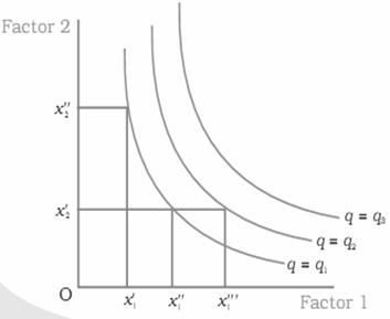 An isoquant is the set of all possible combinations of the two inputs that yield the same maximum possible level of output. Each isoquant represents a particular level of output and is labelled with that amount of output. Cobb-Douglas Isoquants
An isoquant plots all the combinations of two inputs that will produce a given output level. A point on the isoquant curve is technically efficient.In general, isoquants are downward sloping – the more labor we use, the less capital we need. It is bowed inward because of the law of diminishing marginal productivity. In the case of Cobb-Douglas Isoquants inputs are not perfectly substitutable. The slope of an isoquant shows the rate at which L can be substituted for K.
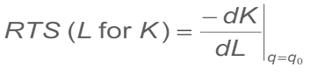
- slope = marginal rate of technical substitution (MRTS).RTS > 0 and is diminishing for increasing inputs of labor. The marginal rate of technical substitution (RTS) shows the rate at which labor can be substituted for capital while holding output constant along an isoquant:
 or
or 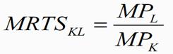
Isoquant map – a set of isoquant curves that show technically efficient combinations of inputs that can produce different levels of output. Leontief Isoquants
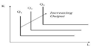
 K and L perfect substitutes perfect complements
Isocost
Isocost line–a line that represents alternative combinations of factors of production that have the same costs. Or in other words, the combinations of inputs (K, L) that yield the producer the same level of output.
The shape of an isoquant reflects the ease with which a producer can substitute among inputs while maintaining the same level of output.
The combinations of inputs that produce a given level of output at the same cost can be expressed as:
wL + rK = C
Rearranging,K= (1/r)C - (w/r)L
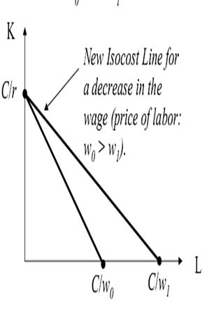
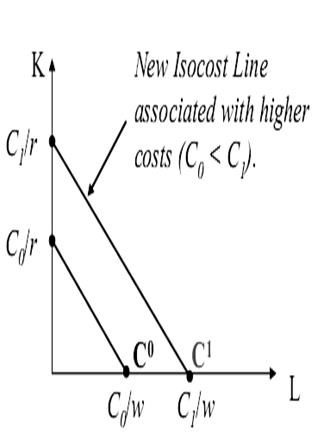
| For given input prices, isocosts farther from the origin are associated with higher costs | Changes in input prices change the slope of the isocost line |
40. Cost minimization (Producer’s choice optimisation)
The least cost combination of inputs for a given output occurs where the isocost curve is tangent to the isoquant curve for that output.
The slopes of the two curves are equal at that point of tangency.
The firm is operating efficiently when an additional output per dollar spent on labor equals the additional output per dollar spent on machines.So that marginal product per dollar spent should be equal for all inputs:
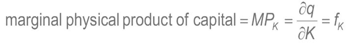
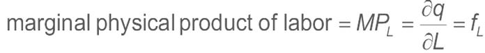
We define marginal physical product as the additional output that can be produced by employing one more unit of that input while holding other inputs constant:
And
Choosing the Economically Efficient Point of Production can be shown in the graph:

Date: 2016-03-03; view: 2449
| <== previous page | | | next page ==> |
| Income and Substitution Effects | | | A large modern corporation |