Supervised learning

In supervised learning, we are given a set of example pairs and the aim is to find a function in the allowed class of functions that matches the examples. In other words, we wish to infer the mapping implied by the data; the cost function is related to the mismatch between our mapping and the data and it implicitly contains prior knowledge about the problem domain.

A commonly used cost is the mean-squared error, which tries to minimize the average squared error between the network's output, f(x), and the target value y over all the example pairs. When one tries to minimize this cost using gradient descent for the class of neural networks called multilayer perceptions, one obtains the common and well-known back propagation algorithm for training neural networks.

Tasks that fall within the paradigm of supervised learning are pattern recognition (also known as classification) and regression (also known as function approximation). The supervised learning paradigm is also applicable to sequential data (e.g., for speech and gesture recognition). This can be thought of as learning with a "teacher," in the form of a function that provides continuous feedback on the quality of solutions obtained thus far.

Unsupervised learning

In unsupervised learning, some data is given and the cost function to be minimized, that can be any function of the data and the network's output, .

The cost function is dependent on the task (what we are trying to model) and our a priori assumptions (the implicit properties of our model, its parameters and the observed variables).

As a trivial example, consider the model where is a constant and the cost 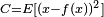. Minimizing this cost will give us a value of that is equal to the mean of the data. The cost function can be much more complicated. Its form depends on the application: for example, in compression it could be related to the mutual information between and , whereas in statistical modeling, it could be related to the posterior probability of the model given the data. (Note that in both of those examples those quantities would be maximized rather than minimized).

Tasks that fall within the paradigm of unsupervised learning are in general estimation problems; the applications include clustering, the estimation of statistical distributions, compression and filtering.

Reinforcement learning

In reinforcement learning, data are usually not given, but generated by an agent's interactions with the environment. At each point in time , the agent performs an action and the environment generates an observation and an instantaneous cost , according to some (usually unknown) dynamics. The aim is to discover a policy for selecting actions that minimizes some measure of a long-term cost; i.e., the expected cumulative cost. The environment's dynamics and the long-term cost for each policy are usually unknown, but can be estimated.

More formally the environment is modeled as a Markov decision process (MDP) with states and actions with the following probability distributions: the instantaneous cost distribution , the observation distribution and the transition , while a policy is defined as conditional distribution over actions given the observations. Taken together, the two then define a Markov chain (MC). The aim is to discover the policy that minimizes the cost; i.e., the MC for which the cost is minimal.

ANNs are frequently used in reinforcement learning as part of the overall algorithm. Dynamic programming has been coupled with ANNs (Neuro dynamic programming) by Bertsekas and Tsitsiklis and applied to multi-dimensional nonlinear problems such as those involved in vehicle routing, natural resources management or medicine because of the ability of ANNs to mitigate losses of accuracy even when reducing the discretization grid density for numerically approximating the solution of the original control problems.

Tasks that fall within the paradigm of reinforcement learning are control problems, games and other sequential decision making tasks.

Learning Algorithms

Training a neural network model essentially means selecting one model from the set of allowed models (or, in a Bayesian framework, determining a distribution over the set of allowed models) that minimizes the cost criterion. There are numerous algorithms available for training neural network models; most of them can be viewed as a straightforward application of optimization theory and statistical estimation.

Most of the algorithms used in training artificial neural networks employ some form of gradient descent. This is done by simply taking the derivative of the cost function with respect to the network parameters and then changing those parameters in a gradient-related direction.

Evolutionary methods, gene expression programming, simulated annealing, expectation-maximization, non-parametric methods and particle swarm optimization are some commonly used methods for training neural networks.

Types of Artificial Neural Networks

Feedforward neural network

The feedforward neural network was the first and arguably most simple type of artificial neural network devised. In this network the information moves in only one direction — forwards: From the input nodes data goes through the hidden nodes (if any) and to the output nodes. There are no cycles or loops in the network. Feedforward networks can be constructed from different types of units, e.g. binary McCulloch-Pitts neurons, the simplest example being the perceptron. Continuous neurons, frequently with sigmoidal activation, are used in the context of backpropagation of error.

Radial basis function network

Radial basis functions are powerful techniques for interpolation in multidimensional space. A RBF is a function which has built into a distance criterion with respect to a center. Radial basis functions have been applied in the area of neural networks where they may be used as a replacement for the sigmoidal hidden layer transfer characteristic in multi-layer perceptrons. RBF networks have two layers of processing: In the first, input is mapped onto each RBF in the 'hidden' layer. The RBF chosen is usually a Gaussian. In regression problems the output layer is then a linear combination of hidden layer values representing mean predicted output. The interpretation of this output layer value is the same as a regression model in statistics. In classification problems the output layer is typically a sigmoid function of a linear combination of hidden layer values, representing a posterior probability. Performance in both cases is often improved by shrinkage techniques, known as ridge regression in classical statistics and known to correspond to a prior belief in small parameter values (and therefore smooth output functions) in a Bayesian framework.

RBF networks have the advantage of not suffering from local minima in the same way as Multi-Layer Perceptrons. This is because the only parameters that are adjusted in the learning process are the linear mapping from hidden layer to output layer. Linearity ensures that the error surface is quadratic and therefore has a single easily found minimum. In regression problems this can be found in one matrix operation. In classification problems the fixed non-linearity introduced by the sigmoid output function is most efficiently dealt with using iteratively re-weighted least squares.

RBF networks have the disadvantage of requiring good coverage of the input space by radial basis functions. RBF centers are determined with reference to the distribution of the input data, but without reference to the prediction task. As a result, representational resources may be wasted on areas of the input space that are irrelevant to the learning task. A common solution is to associate each data point with its own center, although this can make the linear system to be solved in the final layer rather large, and requires shrinkage techniques to avoid overfitting.

Associating each input datum with an RBF leads naturally to kernel methods such as support vector machines and Gaussian processes (the RBF is the kernel function). All three approaches use a non-linear kernel function to project the input data into a space where the learning problem can be solved using a linear model. Like Gaussian Processes, and unlike SVMs, RBF networks are typically trained in a Maximum Likelihood framework by maximizing the probability (minimizing the error) of the data under the model. SVMs take a different approach to avoiding overfitting by maximizing instead a margin. RBF networks are outperformed in most classification applications by SVMs. In regression applications they can be competitive when the dimensionality of the input space is relatively small.

Self-organizing map

The self-organizing map (SOM) invented by Teuvo Kohonen performs a form of unsupervised learning. A set of artificial neurons learn to map points in an input space to coordinates in an output space. The input space can have different dimensions and topology from the output space, and the SOM will attempt to preserve these.

Learning Vector Quantization

Learning Vector Quantization (LVQ) can also be interpreted as a neural network architecture. It was suggested by Teuvo Kohonen, originally. In LVQ, prototypical representatives of the classes parameterize, together with an appropriate distance measure, a distance-based classification scheme.

Recurrent neural network

Contrary to feedforward networks, recurrent neural networks (RNNs) are models with bi-directional data flow. While a feedforward network propagates data linearly from input to output, RNNs also propagate data from later processing stages to earlier stages. RNNs can be used as general sequence processors.

Fully recurrent network

This is the basic architecture developed in the 1980s: a network of neuron-like units, each with a directed connection to every other unit. Each unit has a time-varying real-valued (more than just zero or one) activation (output). Each connection has a modifiable real-valued weight. Some of the nodes are called input nodes, some output nodes, the rest hidden nodes. Most architectures below are special cases.

For supervised learning in discrete time settings, training sequences of real-valued input vectors become sequences of activations of the input nodes, one input vector at a time. At any given time step, each non-input unit computes its current activation as a nonlinear function of the weighted sum of the activations of all units from which it receives connections. There may be teacher-given target activations for some of the output units at certain time steps. For example, if the input sequence is a speech signal corresponding to a spoken digit, the final target output at the end of the sequence may be a label classifying the digit. For each sequence, its error is the sum of the deviations of all activations computed by the network from the corresponding target signals. For a training set of numerous sequences, the total error is the sum of the errors of all individual sequences.

To minimize total error, gradient descent can be used to change each weight in proportion to its derivative with respect to the error, provided the non-linear activation functions are differentiable. Various methods for doing so were developed in the 1980s and early 1990s by Paul Werbos, Ronald J. Williams, Tony Robinson, Jürgen Schmidhuber, Barak Pearlmutter, and others. The standard method is called "backpropagation through time" or BPTT, a generalization of back-propagation for feedforward networks. A more computationally expensive online variant is called "Real-Time Recurrent Learning" or RTRL. Unlike BPTT this algorithm is local in time but not local in space. There also is an online hybrid between BPTT and RTRL with intermediate complexity, and there are variants for continuous time. A major problem with gradient descent for standard RNN architectures is that error gradients vanish exponentially quickly with the size of the time lag between important events, as first realized by Sepp Hochreiter in 1991. The Long short term memory architecture overcomes these problems.

In reinforcement learning settings, there is no teacher providing target signals for the RNN, instead a fitness function or reward function or utility function is occasionally used to evaluate the performance of the RNN, which is influencing its input stream through output units connected to actuators affecting the environment. Variants of evolutionary computation are often used to optimize the weight matrix.

Hopfield network

The Hopfield network (like similar attractor-based networks) is of historic interest although it is not a general RNN, as it is not designed to process sequences of patterns. Instead it requires stationary inputs. It is an RNN in which all connections are symmetric. Invented by John Hopfield in 1982 it guarantees that its dynamics will converge. If the connections are trained using Hebbian learning then the Hopfield network can perform as robust content-addressable memory, resistant to connection alteration.

Boltzmann machine

The Boltzmann machine can be thought of as a noisy Hopfield network. Invented by Geoff Hinton and Terry Sejnowski in 1985, the Boltzmann machine is important because it is one of the first neural networks to demonstrate learning of latent variables (hidden units). Boltzmann machine learning was at first slow to simulate, but the contrastive divergence algorithm of Geoff Hinton (circa 2000) allows models such as Boltzmann machines and Products of Experts to be trained much faster.

Simple recurrent networks

This special case of the basic architecture above was employed by Jeff Elman and Michael I. Jordan. A three-layer network is used, with the addition of a set of "context units" in the input layer. There are connections from the hidden layer (Elman) or from the output layer (Jordan) to these context units fixed with a weight of one. At each time step, the input is propagated in a standard feedforward fashion, and then a simple backprop-like learning rule is applied (this rule is not performing proper gradient descent, however). The fixed back connections result in the context units always maintaining a copy of the previous values of the hidden units (since they propagate over the connections before the learning rule is applied).

Echo state network

The echo state network (ESN) is a recurrent neural network with a sparsely connected random hidden layer. The weights of output neurons are the only part of the network that can change and be trained. ESN are good at reproducing certain time series. A variant for spiking neurons is known as Liquid state machines.

Long short term memory

The long short term memory (LSTM), developed by Hochreiter and Schmidhuber in 1997, is an artificial neural net structure that unlike traditional RNNs doesn't have the vanishing gradient problem. It works even when there are long delays, and it can handle signals that have a mix of low and high frequency components. LSTM RNN outperformed other RNN and other sequence learning methods such as HMM in numerous applications such as language learning and connected handwriting recognition.

References

Date: 2015-12-18; view: 787

References

Date: 2015-12-18; view: 844