CATEGORIES:
BiologyChemistryConstructionCultureEcologyEconomyElectronicsFinanceGeographyHistoryInformaticsLawMathematicsMechanicsMedicineOtherPedagogyPhilosophyPhysicsPolicyPsychologySociologySportTourism
When 8is sufficiently small, the first term is the smaller of the two, and it is well approximated by the expression 1 page
r(x. x + 8)^ \8bmv'(l - x)/v(\ - ,v)"|.
This has a simple interpretation: if the row player demands S more than he should, the column player will resist, and the amount of her resistance is her sample size times the relative loss of utility that she suffers by giving up S of her share. Similarly, if the column player demands S more than she should, the row player's resistance is his sample size times the relative loss of utility that he suffers by giving up S. Thus, the resistance of the transition from the norm (x, 1-х) to the norm (x — S, 1 - x + S) is approximately
r(x. x - S) % Г&»"н'(х)/и(х)1.
Now construct a graph with one vertex for each discrete norm (x. 1 — x), 8 < x < 1 - <5. Denote this vertex by "x." There is a directed edge corresponding to the transition x x - S, and its resistance is approximately ("<5я»т'(х)/1/(х)1. Similarly, the resistance of the directed edgex-* x+ <5 is approximately [<5Ьиг/(1 -х)/г;(1 — x)"|. (The resistance to moving from x to a nonneighboring vertex is at least as great as the resistance to moving to one of the neighboring vertices, hence it turns out that we can ignore these transitions.)
Define the function
/Их) = min{r(x, x + S). r(x, x - 3)}.
By the preceding argument, the resistance to moving to the right, r(x. x + 5), is an increasing function of x, whereas the resistance to moving to the left, r(x. x - 5), is a decreasing function of x. Hence fg(x) is unimodal—first it increases, and then it decreases in x. Let xs be a maximum point of /«(•)• (There are at most two maxima in the set of discrete demands.) For each vertex x such that 5 < x < Xj, select the directed edge (x. x + S), and for each vertex x such that 1 - S > x > Xs, select the directed edge (x, x - 5). Together, these edges constitute an x^-tree, T, because from each vertex other than Xs there is a unique directed path to Xs (see Figure 8.3).
We claim that T is the least resistant rooted tree. To prove this, recall that every rooted tree has exactly one edge that points away from each vertex other than the root. To create the x^-tree T, we chose the least resistant edge exiting from each vertex other than xj. Moreover, each of these edges has a lower (or equal) resistance compared to the least- resistant edge exiting from x$. Hence there cannot be a rooted tree with lower total resistance than T. In fact, this argument shows that any x- tree has higher resistance than T unless x also maximizes /{(■). From
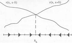 Figure 8.3. The least resistant rooted tree that is rooted at xs.
|
this and theorem 7.1, it follows that the stochastically stable state(s) are precisely those convention(s) hx such that .r maximize(s) fs( ).
When S is small and m is large relative to 8, any maximum хй of f/i(x) lies close to the point x* at which the curves 8amu'(x)/u(x) and 8bmv'( 1 - x)/v(\ - x) intersect, namely,
au\x')/u(x*) = bv'( 1 - x*)/v(l - x'). (8.3)
This is just the first-order condition for maximizing the concave function
я1пи(х)+Mni41 -x), (8.4)
which is equivalent to maximizing
u(x)"v( 1 - x)b. (8.5)
The unique x* that maximizes (8.5) is known as the asymmetric Nash bargaining solution. It follows that xs is arbitrarily close to the asymmetric Nash solution when 8 is sufficiently small and m is sufficiently large relative to 5. This completes the outline of the argument.1
When errors are global, the proof is more complex. The reason is that certain large deviations may have low resistance. Suppose, in particular, that the process is currently in the norm hx. Now suppose that a succession of row players erroneously make the weakest of all demands, 8. This induces the column player to switch to the best reply (1 - 8) provided that the number of errors i satisfies (i/bm)v(\ — 8) > y(l - x), that is,
i > \bmv(l - x)/v(l - 5)1.
When .v is close to 1 the right-hand side is small, that is, the transition from a norm hx to the norm //л has a small resistance. Similarly, the transition from hx (where x is close to zero) to the norm /;t_4 has a small resistance. Nevertheless, it can be shown that when 8 is sufficiently small, this does not fundamentally change the conclusion—namely, that every least resistant x-tree is rooted at a maximum of/«(•). The proof is given in Young (1993b).
Let us illustrate theorem 8.1 with a small example. Suppose that the row players sample one-third of the surviving records and have the utility function u(x) — y/x. Suppose thatthecolumn players sample one- tenth of the surviving records and have the linear utility function v(y) = 1/. The asymmetric Nash solution is (5/8, 3/8), which optimizes (8.5). Let the precision be 8 = .1. When m is large, fs(x)/8m % ч>\(х) л <p2(x), where
<px(x) = <1/3)[1 - u(x - .1 )/н(х)] = (1/3>(1 - y/\ - 1/lOx).
and
4>г(х) = (1/10)[1 - f(l - x - .l)/y(l - д:)] = 1/100(1 - x).
The function <pi {x) л <p2(x) is graphed in Figure 8.4. It achieves its maximum at a value between .6 and .7, and its maximum among the discrete demands occurs at 0.6. Hence the stochastically stable division is (.6, .4).
8.4 Variations on the Bargaining Model
How sensitive are the preceding results to the details of the model? A particularly important ingredient is the structure of the one-shot bargaining game. This game has the slightly unnatural feature that when players ask for too little—that is, when their demands sum to less than unity—the surplus is left on the table. Two natural alternatives suggest themselves. One is to suppose that, when the bargainers demand too little (x + i/ < 1) they split the surplus 1 — x — у equally. The other
approach is to suppose that they only conclude a deal if they coordinate exactly that is, if x + y = 1. The consequences of the latter variation will be taken up in a more general setting in the next chapter. Here we shall briefly examine the first situation.
To keep the argument simple, let us assume that all errors are local and all agents have the same sample size. Suppose that the process is in the norm (x. 1 - x). The payoffs if the row player demands 5 more than the norm, or the column player demands 5 less than the norm, are as follows:
| и(х), 0(1 - X) | н(х + 5/2),о(1 - x-5/2) |
| 0,0 | u(x + 5), о(1 - х-5) |
| 1-х |
| 1 -x-S |
| x x + 5 |
Ignoring the sample size, the reduced resistance to moving from x to

| 0.08 |
| 0.06 |
| 0.04 |
| 0.02 |
| BARGAINING |
| .1 .2 .3 .4 .5 .6 .7 .8 .9 |
| Figure 8.4. The least-resistant rooted tree for the situation S = .1, u(x) = sfx, г>(1 - x) = 1 - лг. |
| I |
•v + 5 is
| r(x. x + <5) = |
I/(x) - 0
(u(x) - 0) + (u(x + 5) - u(x + 5/2))
| (8.6) |
y(l - X) - o(l - X - 5/2)
л
(0(1 - x) - 0(1 - x - 5/2)) + (г;(1 - x - 5) - 0)
126 chapter 8
When <5 is small, we have the approximations
u(x + 8) - u(x + 8/2) % (8/2)u'(x)
and
o(l - x) - o(l - x - 8/2) ъ (<5/2)o'(l - x).
From this we deduce that the first term in (8.6) is much larger than the second, and that
r(x, x + <5) % (5/2)o'(l - *)/o(l - x).
Similarly,
r(x, x-8) = (8/2)u\x)/u(x).
Arguing as before, we deduce that the stochastically stable norms are those that maximize r(x. x — 8) л r(x, x + 8), which are close to the value x* such that o'(l - x)/o(l - x) = u'(x)/u(x). This is the Nash bargaining solution. When the sample sizes differ, a similar argument leads to the asymmetric Nash solution.
8.5 Heterogeneous Populations
Adaptive models lend themselves naturally to the study of heterogeneous populations of agents, as we have already shown in Chapter 5. In the present context, bargainers can differ in at least two dimensions: degree of risk aversion and amount of information. We can therefore characterize each agent by a pair r = (a, u) where 0 < a < 1/2 is the fraction of records the agent samples, and u(x) is a concave, strictly increasing utility function defined for all x € [0.1]. Without loss of generality we can assume that u(0) = 0 and i/(l) = 1. The pair (я, и) represents the agent's type. Let T\ be the set of all types represented among the row players, and let be the set of all types represented among the column players, where both Ti and T2 are finite.
As before, the essence of the problem is to find the least resistance to transiting from any given norm hx to a neighboring norm via local errors. (Indeed, the analysis can be carried out for a more general error structure, as shown in Young (1993b).) When 8 is small and 8m is large,
the resistances to the transitions hx —► hx-/> and lix -» hx+s are given to a good approximation by the expressions
r(x.x-S)^ min [8amu'(x)/u(x))
(в.и)бТ,
and
r(x, л: + S) « min {Sbmv'O. - x)/v(\ - .v)}.
(Ь.р)ет2
When 8 is small and 8m is large, the stochastically stable norms must be close to the unique point x* where these curves cross. In other words, they are close to the point д:* where the lower envelope of the following family of curves achieves its maximum (see Figure 8.5 for an example):
\au'(x)/u(x): (а, и) e 7, | U {bv'(l - x)/v(\ - xy. (b, v) e 72|. (8.7)
Note that (8.7) has a unique maximum whenever the utility functions are concave, positive, and strictly increasing, which we have assumed they are.
| Ч ч |
N
 Figure 8.5. The stable outcome occurs where the lower envelope of the curves attains its maximum.
|
Theorem 8.2 (Young (1993b)). Let G be the discrete Nash demand game with precision 8 played adoptively by two finite populations consisting of types T\
and T2, respectively. /Is S becomes small, the stochastically stable division(s) converge to the unique maximum of
F<(x) = min |au'(x)/u(x). bv'( 1 - x)/v(\ - x)}. (8.8)
«.uleTj |».1>|<Г2
Consider the following example. The row population consists of two types of agents: (я, = 1/4, i<i(x) = x) and (a2 = 1/3, u2(x) = x1/3). The column population consists of two other types of agents: (b] = 1/5, t'i(y) = •/) and (b2 = 1/2. v2(y) = y1/2). Among the row players, the criterion au\x)/u(x) is minimized by the second type of player for every x: a2u'2(x)/u2(x) = l/9x. Among the column players, the criterion bv\y)/v(y) is minimized by the first type of player for every y: biv\(y)/vi(y) = l/5y. Hence F(x) = 1/9* л 1/5(1 - x). It achieves its unique maximum when l/9x = 1/5(1 — x), that is, when x = 5/14. In other words, the stochastically stable division can be made arbitrarily close to (5/14,9/14) for any two populations consisting of the types mentioned above, irrespective of the distribution of these types within each population.
8.6 Bargaining with Incomplete Information
The approach described above is conceptually quite different from the theory of bargaining under incomplete information, which is the standard way of treating heterogeneous populations (Harsanyi and Selten, 1972). In a bargaining model with incomplete information, two agents are drawn at random from their respective populations, and they play a noncooperative game. For simplicity we shall think of this as being the Nash demand game, though Harsanyi and Selten consider a more complicated noncooperative game. Each agent has a belief about the distribution of types in the opposite population, which may or may not correspond to the true distribution of types. An agent's strategy associates a demand with each possible type that he could be. Two strategies form a Bayesian equilibrium if each such demand maximizes the agent's expected payoff (contingent on his type) given his belief about the type of the other agent. Typically there will be a large number of such equilibria for a given set of beliefs. Harsanyi and Selten suggest a set of rational principles for selecting an equilibrium from this set, based on the idea of maximizing the product of the players' payoffs.
In the evolutionary approach, by contrast, agents need not know (or even have beliefs about) the distribution of types in the other population. Instead, they have beliefs about how much their opponent is likely to demand, which they infer empirically from samples of the other side's previous demands. A norm is a situation in which all members of the same population demand the same amount irrespective of their type, and all members of the opposite population demand the complementary amount irrespective of their type. Selection among the norms occurs not by a process of rational choice, but by an implicit process in which norms emerge and are displaced at different rates given the types that are present in each population.
8.7 Fifty-Fifty Division
Under some circumstances it is reasonable to expect that there will be some mixing between the row and column populations. In this case the same types will be present in the two populations, though they may not be present in the same frequencies. This idea can be modeled as follows. Let T = T\ = T2 be the set of all possible types that an agent could be. Let лг(г. r') be the probability that the type pair (r. r') 6 T x T will be chosen to bargain in any given period. The first entry r denotes the row player's type, and the second entry r' denotes the column player's type. The distribution лг mixes roles if every pair in T x T occurs with positive probability. Mixing is a natural consequence of mobility between classes. It also occurs if the classes are rigid but row and column players are drawn from the same "gene pool": in this case, every individual has a positive probability of being any type r, though the probability of being а г may differ for row and column.
When 7Г mixes roles, theorem 8.2 holds as stated with Г] = T2 = T. Since the function F(x) is symmetric about one-half, and since fifty-fifty is a feasible solution for all precisions S, we obtain the following result.
Corollary 8.1. Let G be the discrete Nash demand game with precision S played adoptively by two finite populations in which the roles are mixed. For all sufficiently small s the unique stochastically stable division is fifty-fifty.
Recall that the usual argument for fifty-fifty division is that it constitutes a prominent focal point, which makes it an effective means of coordination (Schelling, 1960). An alternative argument is that fifty-fifty is perceived by many people to be fair, and people derive utility from treating others fairly. Together, these arguments say that fifty-fifty has value both as a coordination device and because it satisfies demands for fairness. However, in economic bargains where parties provide very different inputs (such as land and labor in agriculture) neither of these arguments is especially compelling. When the parties have asymmetric roles and are transparently not equal, fifty-fifty division loses prominence as a focal point and perhaps also its claim to being "fair." Nevertheless, fifty-fifty is in fact quite common in economic bargains between asymmetrically situated agents. In agriculture, for example, equal sharing of the crop is a very common form of contract in many parts of the world, including the midwestern United States.2
The above result provides a different explanation for fifty-fifty (and, more generally, for equal division of the surplus over and above the parties' disagreement outcomes). When bargainers are drawn from a given population of types, and their expectations are shaped by precedent, equal division is the most stable convention over time. Once established, it is the hardest to dislodge. Interpreted in this way, equal division may be a focal point because it is stable, not the other way around.
Chapter 9
CONTRACTS
THE PRECEDING chapter examined the effect of adaptive learning on a particular form of contract, namely, the division of a fixed pie. Here we shall extend the analysis to the evolution of contracts more generally. By a contract, we mean the terms that govern a relationship between people. Contracts may be written or unwritten, explicit or implicit. Some contracts are spelled out in fine detail, such as rental contracts between tenants and landlords or lending agreements between bankers and borrowers. Others are mostly implicit, such as the common understandings that a couple brings to a marriage. Still others occupy a middle ground: employment contracts are usually explicit about some matters, such as the number of hours to be worked, but quite vague about others, such as the relationship between performance and pay.
Whether the terms are implicit or explicit, what matters for the durability of a contract is that the parties know what is expected of them under various contingencies, and that behavior be consistent with expectations. This creates a demand for standard or conventional contracts that have been tested by experience, since the parties have a clearer idea about what their terms mean and how they will play out under different circumstances. Moreover, the existence of standard contracts makes it easier for the parties to come to terms in what would otherwise be a complex and perhaps indeterminate bargaining situation.
At the individual level we can model the choice of contract as a pure coordination game. The terms that a player demands are governed by his or her expectations about the terms that the other side will demand, and these expectations are governed by observations about the terms that agents in the other population actually did demand in previous periods. We further assume that the learning process is buffeted by small stochastic perturbations that represent idiosyncratic behavior and other minor disturbances. This learning process has quite striking implications for the welfare properties of contracts that are likely to be prevalent in the long run. Specifically, we shall show that adaptive learning tends to select contract forms that are efficient—the expected payoffs lie on the Pareto frontier. Furthermore, the payoffs from such contracts tend to be centrally located on the Pareto frontier instead of near the boundaries. When the payoffs form a discrete approximation of a convex set, the stochastically stable contract gives the parties approximately equal payoffs relative to the payoffs they could get under their most preferred contracts. Interpreted in the context of economic and social institutions, this says that the most stable contractual arrangements are those that are efficient, and more or less egalitarian, given the parties' payoff opportunities.
9.1 Choice of Contracts as a Coordination Game
Consider two disjoint classes of individuals—A and В—who can enter into relationships with each other. They might consist, for example, of employers and employees, men and women, owners and renters, or creditors and debtors. For simplicity, we shall assume that each relationship involves a pair of individuals, and that the terms of their relationship can be expressed in a finite number of alternative contracts. Let ak be the expected payoff to the A-players from the kth contract, and b< the expected payoff to the B-players, 1 < к < K. We assume that these payoffs represent the players' choices under uncertainty, and that they satisfy the usual von Neumann-Morgenstern axioms. We shall also suppose that everyone knows his or her own payoff, but we need not suppose that anyone knows anyone else's payoff.
At the beginning of each period, a pair of players is drawn at random from A x B, and each of them names one of the К contracts. If they name the same one, they enter into a relationship on those terms, and their expected payoffs are (<?ь b/t)- If they name different contracts, they are unattached until the next matching. We shall assume that all contracts are desirable, that is, that the expected payoff from any feasible contract is strictly higher for both parties than the expected payoff from being unattached. Without loss of generality, we may normalize each player's utility function so that the payoff from the unattached state is zero. The recurrent game is therefore а К x К pure coordination game in which the diagonal payoffs are positive and the off-diagonal payoffs are zero. Indeed, the analysis below applies to any pure coordination game, whether or not it arises in this way.
Let P"' s-' be adaptive learning applied to this situation. As usual, the error term reflects the idea that players sometimes make choices for idiosyncratic reasons that lie outside the model. Although these un
conventional, quirky choices often result in missed opportunities with the more conventionally minded (and therefore quirky people are more likely to be unattached), if enough such choices accumulate, they can cause society to tip into a new norm. For the present, we shall assume (as in previous chapters) that these idiosyncratic shocks are independently and identically distributed among agents. In Section 9.7, we shall show that even when the shocks are correlated, the long-run outcome remains the same provided that the degree of correlation is not too large.
9.2 Maximin Contracts
A contract is efficient if there exists no other contract that yields higher payoffs to both parties. It is strictly efficient if there is no other contract that yields at least as high a payoff to one party and a strictly higher payoff to the other. Let a+ = max* я* be the maximum payoff to the A-players under some contract; similarly let b+ be the maximum payoff to the B-pIayers. There is no loss of generality in scaling the utility functions so that a+ = b+ = 1, and we shall assume henceforth that this normalization has been made. Define the welfare index of contract к to be the smaller of ak and bk,
wk= fljt л bk. (9.1)
and let
w+ = max wk. (9.2)
к
A contract with welfare index w+ will be called a maximin contract. A maximin contract favors the least-favored class in the sense that no other contract yields a higher expected payoff to the class that is least well-off relative to its most-preferred contract.
Figure 9.1 illustrates the welfare indices of eight different contracts, together with the maximin contract. The intersection of the dotted lines with the diagonal determine the welfare indices, and w+ is the value that lies furthest out along the diagonal.
| Pavoff to class 2 |
| Index |
| _ (1,-2) |
| Figure 9.1. Welfare indices for eight contracts. |
| Payoff to class 1 |
Why, though, is it meaningful to compare von Neumann-Morgenstern utilities in this way? From the individual's perspective, it is not meaningful, but we do not assume that individuals make such comparisons. (How could they if they do not know the others' utility functions?) The claim is that society makes interpersonal comparisons through the feedback effect of precedents on expectations. Moreover, there is a simple explanation for this phenomenon: individuals choose actions based on their payoffs times the probabilities with which they expect the other side to choose these same actions. In a stochastic environment, this means that individuals with different utility functions adjust their choice behavior at different rates. Interpersonal comparisons therefore arise implicitly because differences in von Neumann-Morgenstern utility imply different rates of behavioral adaptation in a stochastic environment. At the societal level, this creates a selection bias in favor of the maximin norm, or something close to it, as we shall now show.
9.3 A Contract Selection Theorem
| (9.3) |
To formulate our result precisely, we need some further notation. Let a~ denote the lowest payoff to the A players among all contracts in which the В players get their maximum, and define b~ similarly (see Figure 9.1). Let
iv = a v b
Normally we would expect w~ to be small, because eking out the maximum possible gain for one class will generally occur at the expense of the other class as a result of substitution possibilities. We claim that the smaller w~ is, the closer is the stochastically stable outcome to the maximin solution. Specifically, define the distortion parameter a as
a = нГ(1 - (м>+)2)/(1 + w~)(w+ + w~). (9.4)
Note that a is small when w~ is small and/or w+ is close to one.
Theorem 9.1. Let G be a two-person pure coordination game, and let P": f r be adaptive play. If s/nt is sufficiently small, every stochastically stable state is a convention; moreover, if s is sufficiently large, every such convention is efficient and approximately maximin in the sense that its welfare index is at least (w+ -ct)/( 1 + a).
The usefulness of this lower bound depends on the problem at hand. In the example shown in Figure 9.1, w+ = .700 and w~ = .200, so or = .067. The theorem therefore says that the stochastically stable outcome has welfare index at least (.700 - ,067)/1.067 = .593. It is evident from the figure that the only contract that satisfies this criterion is the maximin contract. If there were other contracts with welfare index between .593 and .700, the theorem would not eliminate them; in general, however, the addition of more contracts will tend to increase w+ and to decrease w~, which reduces a and correspondingly increases the cutting power of the theorem.
While theorem 9.1 does not provide the sharpest possible lower bound in all coordination games, it is best possible for some games, as we show by example in Section 9.5. There are important classes of games, moreover, for which the stochastically stable outcome is essentially the same as the maximin solution. These include 2x2 coordination games, symmetric coordination games, and coordination games whose payoffs form a discrete approximation of a convex bargaining set. Indeed, in the latter case the stochastically stable outcome is the Kalai-Smorodinsky solution, as we show in Section 9.7.
The general approach to computing the stochastically stable outcome relies on the methods developed in previous chapters. Specifically, equation (7.2) shows that the resistance to transiting from coordination equilibrium j to coordination equilibrium к (as a function of the sample 136 chapter 9
size s) is given by the expression
r-jt = Г5Г/Л, where rjk = я,/(я, + я*) л Ь,/(Ь; + bk). (9.5)
We then apply the method of rooted trees to determine the equilibrium with minimum stochastic potential, as described in Chapter 3.
9.4 The Marriage Game
Let us illustrate these ideas with an example involving marriage contracts. It is a commonplace observation that men and women often play different roles in a marriage, and that these differences depend to a substantial extent on social custom. Marital arrangements that are normal and customary in Papua New Guinea may not be normal or customary in Sweden, for example. Furthermore, social expectations about these matters change over time. In Europe and the United States, for example, the rights of married women have evolved markedly over the past two hundred years from a situation where they enjoyed very little autonomy to one that more closely approximates equality. This change resulted from gradual shifts in attitudes and expectations in the general population, rather than from any single defining event; hence it has a distinctly evolutionary flavor. While the theory described above is not intended to explain such historical developments in detail, it can nevertheless shed light on a related question: in partnerships between people who are complementary in some respect, what distribution of rights within the partnership is the most stable over the long run?
Date: 2016-04-22; view: 713