CATEGORIES:
BiologyChemistryConstructionCultureEcologyEconomyElectronicsFinanceGeographyHistoryInformaticsLawMathematicsMechanicsMedicineOtherPedagogyPhilosophyPhysicsPolicyPsychologySociologySportTourism
CHAPTER 9. Contracts 131 4 page
If the two players were actually playing the mixed equilibrium in each period, the row player would choose A and В with probabilities 1/(1 + ,/2) and v/2/(l + J2), while the column player would independently choose A and В with probabilities v/2/(l + ^2) and 1/(1 + J2). Thus the probability of coordination would be 2,/2/(l + ,/2)2 and the expected payoff to each player would be J2/(\ + J2). Thus, while the time-average behavior of the players in fictitious play is converging to the mixed equilibrium, this does not reflect what they are doing period-by-period.
2.4 Potential Games
Let us introduce another class of games for which fictitious play is well behaved, and that will play a role in future chapters.9 Let G be an n-
person game with finite strategy sets X]. X2.......... X„ and utility functions
Uj". X —* R, where X = X,. G is a (weighted) potential game if there exists
a function p: X —► R and positive real numbers А]. Л2.......... X„ such that
for every i, every e X_/, and every pair x„ x- G X„
AiUi(Xi, X-i) - XjUjtfj, x-i) = p(Xj. x-i) - p(x't, x-i). (2.10)
In other words, the utility functions can be rescaled so that whenever a player changes strategy unilaterally, the change in his or her utility
equals the change in potential. The point here is that the same potential function p applies to all players. In particular, suppose that the players choose some н-tuple of actions x° e X. A path of unilateral deviations
(UD-path) is a sequence of form x°, x1.............. xk, where each x' e X, and
xi differs from its predecessor x'"1 in exactly one component. Given distinct н-tuples x and x', there will typically exist multiple UD-paths from x to x'. If G is a potential game, the total change in (weighted) utility along such a path, summed over all deviating players, must be the same independently of the path taken.
The most transparent example of a potential game is a game with identical payoff functions u,(x) = u(x) for every player i. A considerably less obvious example is the following class of Cournot oligopoly games. Consider n firms with identical cost functions c(cji), where c(q,) is continuously differentiable in <7, and <7, is the quantity produced by firm i. Let Q = J^ q„ and suppose the inverse demand function takes the form P — a - bQ, where P is the unit price and a, b > 0. Then the profit for firm i (which we identify with i's payoff) is
"((<?! • 12.... qn) = (a- bQ)qi - c(qi).
It is straightforward to check that the following is a potential function for this game:
(2.11)
| 1=1 |
| i=l |
\<i<j<m i=l
As a third example, we claim that every symmetric 2x2 game is a potential game. Indeed, the payoffs from such a game can be written in the form
А В
| a, a | с, d |
| d, с | b.b |
| (2.12) |
| A В |
| (2.13) |
It is easy to see that a potential function for this game is
p(A, A) = a - d p(A, В) = 0 p(B, A) = 0 p(В, B) = b - c.
We claim that every weighted potential game possesses at least one Nash equilibrium in pure strategies. To see this, consider any strategy- tuple x° e X. If x° is not a Nash equilibrium of G, there exists a player i who can obtain a higher payoff by changing to some strategy xj ф x®. Continuing in this manner, one generates a finite improvement path,
namely, a UD-path x°, x1______ xk such that the unique deviator at each
stage strictly increases his utility. It follows that the potential is strictly increasing along any finite improvement path. Since the strategy space X is finite, the path must end at some x* e X from which no further deviations are worthwhile; that is, x* is a pure Nash equilibrium of G." The following result shows that in a potential game, fictitious play always converges to the set of Nash equilibria (whether pure or mixed).
THEOREM 2.4 (Monderer and Shapley, 1996b). Every weighted potential game has the fictitious play property.
2.5 Nonconvercence of Fictitious Play
Many games do not have the fictitious play property, however. The first such example is due to Shapley (1964), and can be motivated as follows.
The Fashion Game
Individuals 1 and 2 go to the same parties, and each pays attention to what the other wears. Player 1 is a fashion follower and likes to wear the same color that player 2 is wearing. Player 2 is a fashion leader and likes to wear something that contrasts appropriately with what player 1 is wearing. For example, if player 1 is wearing red, player 2 prefers to wear blue (but not yellow); if player 1 is wearing yellow, player 2 prefers red, while if player 1 dons blue, player 2 wants to be in yellow. The payoff matrix has the following form:
Player 2 Red Yellow Blue
| 1,0 | 0,0 | 0,1 |
| 0,1 | 1,0 | 0,0 |
| 0,0 | 0,1 | 1,0 |
| Red Player 1 Yellow Blue |
This game has a unique Nash equilibrium in which the players take each action with probability 1/3.
Assume now that both players use fictitious play as a learning rule, and that they both start by wearing red in the first period. The process then unfolds as follows (we assume that ties are broken according to the hierarchy yellow > blue > red).
t
1 2 3 4 5 6 7 8 9 10 11 12 13 14...
Player 1 RRBBBBBYYY Y Y YY Player 2 RBBBYYYYY Y Y Y YR
Roughly speaking, the process follows the fashion cycle red —» blue yellow —> red, with player 2 leading the cycle, and player 1 following. More precisely, define a run to be a sequence of consecutive periods in which neither player changes action. The runs in the above sequence follow the cyclic pattern shown below.
| R R |
| Y R |
| R В |
| Y Y |
| В В |
| В Y |
Moreover, the number of periods in each consecutive cycle grows exponentially. Let p'j = (p'lK, p'tY, p'jB) be the relative frequency with which player i (;' = 1.2) plays each strategy up through time t. Shapley (1964) showed that (p\,p'2) does not converge to the Nash equilibrium; instead, it converges to a cycle in the product space Д3 x Д3, where лз = {(</ь (?2.<?з) 6 R3: £<7, = 1}.
While this example might suggest that fictitious play has its drawbacks as a learning rule, it also suggests that equilibrium has its drawbacks as a solution concept. Fashion would not be fashion if it were not constantly in flux. It is a form of interaction in which we expect cyclic behavior.12 The fact that fictitious play cycles in such a game might be seen as an argument in its favor, since cycling in this case is at least as plausible as Nash equilibrium behavior.
There are other games, however, in which Nash equilibrium is more clearly the "right" solution, yet fictitious play fails to find it. Define a two-person coordination game to be a game in which each player has the same number of actions, which can be indexed so that it is a strict Nash equilibrium for the players to- play actions having the same index. In other words, let the actions of the players be indexed j = 1,2,..., m, and let the payoff from playing the pair of actions with indices (/. k) be ajk for the row player and b^ for the column player. In a coordination game, ац > л*7 and Ьц > Ьц for every distinct pair of indices j and k. Consider the following example, drawn from Foster and Young (1998).
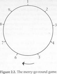
The Merry-Go-Round Game
Rick and Cathy are in love, but they are not allowed to communicate. Once a day, at an appointed time, they can take a ride on a merry-go- round, which has nine pairs of horses (Figure 2.2). Before taking a ride, each chooses one of the pairs without communicating his or her choice to the other. There are no other riders. If they book the same pair they get to ride side by side, which is their preferred outcome. If they choose different pairs, their payoffs depend on how conveniently they can look at each other. If Rick sits just behind Cathy, then he can see her but she has trouble looking at him, because the horses all face in the clockwise direction. Say this outcome has payoff 4 for Rick and payoff 0 for Cathy. If they are on opposite sides of the circle, they can both see each other easily, but the one who has to crane his or her neck less has a slightly higher payoff (5 compared to 4). If they sit side by side, they can look at each other to their hearts' content, which has a payoff of 6 for both. The payoff matrix is therefore as follows:
| 6,6 | 4,0 | 4,0 | 4,0 | 5,4 | 4,5 | 0,4 | 0,4 | 0,4 |
| 0,4 | 6,6 | 4,0 | 4,0 | 4,0 | 5,4 | 4,5 | 0,4 | 0,4 |
| 0,4 | 0,4 | 6,6 | 4,0 | 4,0 | 4,0 | 5,4 | 4,5 | 0,4 |
| 0,4 | 0,4 | 0,4 | 6,6 | 4,0 | 4,0 | 4,0 | 5,4 | 4,5 |
| 4,5 | 0,4 | 0,4 | 0,4 | 6,6 | 4,0 | 4,0 | 4,0 | 5,4 |
| 5,4 | 4,5 | 0,4 | 0,4 | 0,4 | 6,6 | 4,0 | 4,0 | 4,0 |
| 4,0 | 5,4 | 4,5 | 0,4 | 0,4 | 0,4 | 6,6 | 4,0 | 4,0 |
| 4,0 | 4,0 | 5,4 | 4,5 | 0,4 | 0,4 | 0,4 | 6,6 | 4,0 |
| 4,0 | 4,0 | 4,0 | 5,4 | 4,5 | 0,4 | 0,4 | 0,4 | 6,6 |
|
A similar story can be told for two players who want to coordinate on some date in the calendar. For example, think of two car manufacturers who announce their new models once a year. If they announce on the same date, they generate a lot of media coverage. If one announces "earlier" than the other does, they receive less publicity in total, and the earlier announcement casts a "publicity shadow" on the later one. In other words, miscoordination hurts both parties but it hurts one party more than the other.
When players try to learn such a game by fictitious play, they can fall into a cyclic pattern in which they keep locating on (more or less) opposite sides of the circle, and never coordinate. That is, under certain initial conditions, the distribution of the other person's previous actions are such that each player would rather advance one position (to get a better view of the other) than try to coordinate exactly, which carries the risk of "missing" by one position.
2.6 Adaptive Play
One might wonder why the players are not clever enough to figure out that they are caught in a cycle. Perhaps if they analyzed the data in a more sophisticated way, they would avoid falling into such a trap. We shall not pursue this avenue further here, although it is certainly one that should be pursued. Let us recall, however, that the situation we have in mind is a recurrent game played by a changing cast of characters who have limited information, have only modest reasoning ability, are short-sighted, and sometimes do unexplained or even foolish things. Such players may be quite unable to make sophisticated forecasts; nevertheless they may be able to feel their way collectively toward interesting and even sensible solutions. Indeed, this is the case when the players are even less rational and less well-informed than they are in fictitious play.
To make these ideas precise, let us fix an н-person game with finite
strategy sets Xi.......... X„. The joint strategy space is X = f[ X„ and the
payoff functions are ;<,: X —* R. In each period, one player is drawn at
random from each ofn disjoint classes Ci, C2............. C,„ to play the game
G. Let x'j e X, denote the action taken by the i player at time /. The
play, or record, at time t is the vector x' = (x\, x'2.......................... x'n). The state of
the system at the end of period t is the sequence of the last m plays: h1 = (x'~m+1,..., *'). The value of m determines how far back in time the players are willing (or able) to look.
Let X'" denote the set of all states, that is, the set of all histories of length m. The process starts out in an arbitrary state h° consisting of m records. Given that the process is in state h' at the end of period t, consider some player who is selected to play role i in period t + 1. Each player has access to information about what some of the previous players have done, which is relayed through established networks of friends, neighbors, co-workers, and so on. In other words, access to information is part of an agent's situation, not the result of an optimal search. We model the information transmission process as a random variable: the current i player draws a sample of size s from the set of actions taken by each of the other role players over the last m periods. These n — 1 samples are drawn independently. Let p':j € Д, denote the sample proportion of j's actions in i's sample, and let p'_t = П/^iP!,- (a "hat" over a variable indicates that it is a random variable.)
Idiosyncratic behaviors are modeled as follows. Let e > 0 be a small positive probability called the error rate. With probability 1-f the/player chooses a best reply to p'_, and with probability e he chooses a strategy in Xj at random. If there are ties in best reply, we assume each is chosen with equal probability.1" These errors correspond to mutations in biological models of evolution. Here, they are interpreted as minor disturbances to the adaptive process, which include exogenous stochastic shocks as well as unexplained variation (idiosyncracies) in personal behavior. The probability of making an error is assumed to be independent across players. Taken together, these factors define a Markov process called adaptive play with memory m, sample size s, and error rate e (Young, 1993a). This model has four key features: bounded!}/ rational responses to forecasts of others' recent behavior, which are estimated from limited data and are perturbed by stochastic shocks. In the following chapters, we shall examine the properties of this process in detail, and show how it leads to a new concept of equilibrium (and disequilibrium) selection in games.
Chapter 3
DYNAMIC AND STOCHASTIC STABILITY
3.1 Asymptotic Stability
Before analyzing the dynamic behavior of the learning model introduced in the preceding chapter, we need a framework for thinking about the asymptotic properties of dynamic systems in general. Let Z denote a set (finite or infinite) of possible states of a dynamical system. For analytical convenience, we shall assume that Z is contained in a finite Euclidean space Rk. A discrete-time dynamical process is a function £(/. z)
defined for all discrete times t = 0.1. 2,3________ and all z in Z such that
if the process is in state z at time t, then it is in state z' = f(f. z) at time t + 1. From any initial point z° the solution path of the process is {z^z1 = f (0, z°), z2 = f(1. z1),...).
There are two senses in which a state z can be said to be "stable" in such a process. The weaker condition (Lyapunov stability) says that there is no local push away from the state; the stronger condition (asymptotic stability) says that there is a local pull toward the state. Formally, a state z is Lyapunov stable if every open neighborhood В of z contains an open neighborhood of z such that any solution path that enters stays in В from then on. In particular, the process need not return to z, but if it comes close to z it must remain close. A state z is asymptotically stable if it is Lyapunov stable and the open neighborhood B° can be chosen so that if a solution path ever enters then it converges to z.
Although most of the processes considered in this book take place in discrete time, we shall briefly outline the analogous ideas for continuous- time processes. Let Z be a compact subset of Euclidean space Rk. A continuous-time dynamical process is a continuous mapping R x Z —► Z where for all z° 6 Z, £(0, z°) = z° and f(f,z°) represents the position of the process at time t given that it started at z°. Such a system often arises as the solution to a system of first-order differential equations of the form
z = ф(г) where ф: Z Rk. (3.1)
Here ф defines the vectorfield, that is, the direction and velocity of motion at each point in Z. A solution to (3.1) is a function R x Z —*■ Z such that
d$(t, z)/dt = 0[£(f, 2)] for all t 6 R and z e Z. (3.2)
The function ф is Lipscliitz continuous on a domain Z* if there exists a nonnegative real number L (the Lipschitz constant) such that |$(z) - <p(z')\ < L\z-z'\ for all z, z'eZ*. A fundamental theorem of dynamical systems states: l/ф is Lipschitz continuous on an open domain Z* containing Z, then for every z° e Z there exists a unique solution £ such that%( 0, z°) = z°; moreover t;(t, z°) is continuous in t and z0.1
To illustrate asymptotic stability in the discrete case, consider the dynamics defining fictitious play:
*« _ (3.3,
Although we derived this equation for 2 x 2 games, the same equation holds for any finite «-person game G with an appropriate rule for resolving best-reply ties.
Let x* e X be a strict Nash equilibrium, that is, x* is the unique best reply to x'_j for every player i. Since the utility functions и,: Д —> R are continuous, there exists an open neighborhood Bx- of x* such that x* is the unique best reply to p_, for all p e Bx-. From this and (3.3), it follows that every strict Nash equilibrium is asymptotically stable in the discrete-time fictitious play dynamic. The same holds for the continuous-time version of the best-reply dynamic (2.9). In particular, every coordination equilibrium of a coordination game is asymptotically stable in the discrete (or continuous) form of the best-reply dynamic.
A similar result holds for a much larger class of learning dynamics, including the replicator dynamic. Let Д = f] д< be the space of mixed strategies for a finite «-person game G. Imagine that each population of players forms a continuum, and that at each time t, each player has an action, which he or she plays against randomly drawn members of the other populations. We can represent the state at time t by a vector PC) <= Д, where p,*(f) denotes the proportion of population i playing the fcth" action in X, and к indexes the actions in X,. A growth rate dynamic is a dynamical system of form
Pik = gik(p)pik where pi ■ g,(p) = 0 and £,: Д Д,. (3.4)
The condition p,gi(p) = 0 is needed to keep the process in the simplex Д, for each i. Let us assume that, for every /', g, is Lipschitz continuous on an open domain containing A, so that the system has a unique solution from any initial state pa. (Such a process is sometimes called a regular selection dynamic.) The function g,k(p) expresses the rate at which the proportion of population i playing the /cth action in X^ increases (or decreases) as a function of the current state p e A. Note that an action cannot grow if it is not present in the population. A particular consequence is that every vertex of Д (every /(-tuple x <= X) is a rest point of the dynamic.
Let Xjk denote the /cth action of player i. The dynamic is payoff mono- tonic if in each state, the growth rates of the various actions are strictly monotonic in their expected payoffs.2 In other words, for all p G Д, all i, and all кфк,
itiiXik. p-i) > т(хц". p-i) iff gik(p) > git(p). (3.5)
The replicator dynamic is the special case in which the growth rate of each action Xjk equals the amount by which its payoff exceeds the average payoff to members of population i, that is,
Pik = [Ui(xik,p-i) - Uj(p)]plk. (3.6)
It can be shown that in a payoff monotonic, regular selection dynamic, every strict Nash equilibrium is asymptotically stable. Thus if the game has multiple strict Nash equilibria (as in a coordination game), the dynamics can "select" any one of them, depending on the initial conditions.3
3.2 Stochastic Stability
Even though asymptotic stability is essentially a deterministic concept, it is sometimes invoked as a criterion of stability in the presence of random perturbations. To illustrate, suppose that a process is in an asymptotically stable state and that it receives a small, one-time shock. If the shock is sufficiently small, then by the definition of asymptotic stability the process will eventually revert to its original state. Since the impact of the shock ultimately wears off, one could say that the state is stable in the presence of stochastic perturbations. The difficulty with
this argument is that, in reality, stochastic perturbations are not isolated events. What happens when the system receives a second shock before it has recovered from the first, then receives a third shock before it has recovered from the second, and so forth? The concept of asymptotic stability is inadequate to answer this question.
In the next two sections, we introduce an alternative concept of stability that takes into account the persistent nature of stochastic perturbations. Instead of representing the process as a deterministic system that is occasionally tweaked by a random shock, we shall represent it as a stochastic dynamical system, in which perturbations are incorporated directly into the equations of motion. Such perturbations are a natural feature of most adaptive processes, including those discussed in the preceding chapter. For example, the replicator dynamic amounts to a continuous approximation of a finite process in which individuals from a finite population reproduce (and die) with probabilities that depend on their payoffs from interactions. In models of imitation, the random component follows from the assumption that individuals update their strategies with probabilities that are payoff dependent. In reinforcement models, agents are assumed to choose actions with probabilities that depend on the payoffs they received from these actions in the past. And so forth. Virtually any plausible model of adaptive behavior we can think of has stochastic components.
Although previous authors have recognized the importance of stochastic perturbations in evolutionary models, it has been standard to suppress them on the grounds that they are inherently small, or else small in the aggregate because the variability is averaged over many individuals, and to study the expected motion of the process as if it were a deterministic system. While this may be a reasonable approximation of the short -run (or even medium-run) behavior of the process, however, it may be a very poor indicator of the long-run behavior of the process. A remarkable feature of stochastic dynamical systems is that their long- run (asymptotic) behavior can differ radically from the corresponding deterministic process no matter how small the noisj term is. The presence of noise, however minute, can qualitatively alter the behavior of the dynamics. But there is also an unexpected dividend: since such processes are often ergodic, their long-run average behavior can be predicted much more sharply than that of the corresponding deterministic dynamics, whose motion usually depends on the initial state. In the next several sections we shall develop a general framework for analyzing these issues. We shall then apply it to adaptive learning, and show how it leads
to a theory of equilibrium (and disequilibrium) selection for games in general.
3.3 Elements of Markov Chain Theory
A discrete-time Markov process on a finite state space Z specifies the probability of transiting to each state in Z in the next period, given that the process is currently in some given state z. Specifically, for every pair of states z, т! e Z, and every time t > 0, let Pa'(f) be the transition probability of moving to state z' at time t + 1 conditional on being in state г at time t. If P& = Ргг'(0 is independent of t, we say that the transition probabilities are time homogeneous. This assumption will be maintained throughout the following discussion.
Suppose that the initial state is 2°. For each t > 0, let p'(z \ z°) be the relative frequency with which state z is visited during the first t periods. It can be shown that as t goes to infinity, p'(z \ z°) converges almost surely to a probability distribution д°°(2 | 2°), called the asymptotic frequency distribution of the process conditional on г0.4 The distribution can be interpreted as a selection criterion: over the long run, the process selects those states on which p 00(2 | 2°) puts positive probability. Of course, the state or states that are selected in this sense may depend on the initial state, 2°. If so, we say that the process is path dependent, or nonergodic. If the asymptotic distribution px(z | 2°) is independent of 2°, the process is ergodic.
Consider a finite Markov process on Z defined by its transition matrix, P. A state z' is accessible from state z, written z —> z', if there is a positive probability of moving from г to z' in a finite number of periods. States 2 and z' communicate, written z ~ z', if each is accessible from the other. Clearly ~ is an equivalence relation, so it partitions the space Z into equivalence classes, which are known as communication classes. A recurrent class of P is a communication class such that no state outside the class is accessible from any state inside it. It is straightforward to show that every finite Markov chain has at least one recurrent class.
Denote the recurrent classes by Ej. E2............. EK. A state is recurrent if it is
contained in one of the recurrent classes; otherwise it is transient. A state is absorbing if it constitutes a singleton recurrent class. If the process has exactly one recurrent class, which consists of the whole state space, the process is said to be irreducible. Equivalently, a process is irreducible if and only if there is a positwe probability of moving from any state to any other state in a finite number of periods.
The asymptotic properties of finite Markov chains can be studied
1 ebraically as follows. Let z\.......... Zn be an enumeration of the states,
and let p be a probability distribution on Z written out as a row vector: _ p(zi) /i(ZN))- Consider the system of linear equations
цР = д, where ц > 0 and ^ m(z) = 1. (3.7)
2€Z
It can be shown that this system always has at ieast one solution ц, which is called a stationary distribution of the process P. The term stationary is apt for the following reason. Suppose that ц (z) is the probability of being in state z at some time t. The probability of being in state z at time t + 1 is the probability (summed over all states w) of being in state w at time t and transiting to z in the next period. In other words, the probability of being in state z in period t +1 equals p(w)Pwz. Equation (3.7) states that this probability is precisely p(z) for every z € Z. In other words, if H is the probability distribution over states at some time t, then д is also the probability distribution over states at all subsequent times.
Date: 2016-04-22; view: 822
| <== previous page | | | next page ==> |
| CHAPTER 9. Contracts 131 2 page | | | CHAPTER 9. Contracts 131 5 page |