CATEGORIES:
BiologyChemistryConstructionCultureEcologyEconomyElectronicsFinanceGeographyHistoryInformaticsLawMathematicsMechanicsMedicineOtherPedagogyPhilosophyPhysicsPolicyPsychologySociologySportTourism
Motion in Two or Three Dimensions
This chapter extends the material of the preceding two chapters to two and three dimensions. Many of the ideas of previous chapter, such as position, velocity, and acceleration, are used here, but they are now a little more complex because of the extra dimensions.
1.2 Position and Displacement
One general way of locating a particle (or particle-like object) is with a position vector  , which is a vector that extends from a reference point (usually the origin of a coordinate system) to the particle. In the unit-vector notation, can be written
 , (4-1)
where  ,
,  , and
, and  are the vector components of , and the coefficients
  ,
,  , and
, and  are its scalar components.
The coefficients , , and give the particle's location along the coordinate axes and relative to the origin; that is, the particle has the rectangular coordinates ( , , ). For instance, Fig. 4-1 shows a particle with position vector
 (4-2)
(4-2)
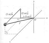 Fig. 4-1
|
and rectangular coordinates  . Along the axis the particle is 3 m from the origin, in the
  direction. Along the axis it is 2 m from the origin, in the
  direction. Along the axis it is 5 m from the origin, in the
  direction.
As a particle moves, its position vector changes in such a way that the vector always extends to the particle from the reference point (the origin). If the position vector changes, say, from  to
to  during a certain time interval, then the particle's displacement
  during that time interval is
 (4-2)
(4-2)
Using the unit-vector notation, we can rewrite this displacement as

or as
 (4-3)
(4-3)
where coordinates (  ,
,  ,
,  ) correspond to position vector and coordinates (
  ,
,  ,
,  ) correspond to position vector . We can also rewrite the displacement by substituting
  for
for  ,
,  for
for  , and
, and  for
for  :
:
 (4-3)
(4-3)
Example 4-1
In Fig. 4-2, the position vector for a particle is initially

 Fig. 4-2
|
and then later is
 .
.
What is the particle's displacement from to ?
Solution. The Key Idea is that the displacement is obtained by subtracting the initial position vector from the later position vector . That is most easily done by components:
 (Answer)
This displacement vector is parallel to the  plane, because it lacks any component, a fact that is easier to see in the numerical result than in Fig. 4-2.
Sample Problem 4-2
A rabbit runs across a parking lot on which a set of coordinate axes has been drawn. The coordinates of the rabbit's position as functions of time  are given by
 (4-5)
(4-5)
And  , (4-6)
with in seconds and and in meters.
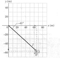
(a) At  s, what is the rabbit's position vector in unit-vector notation and as a magnitude and an angle?
Solution. The Key Idea here is that the and coordinates of the rabbit's position, as given, are the scalar components of the rabbit's position vector . Thus, we can write
|
(We write  rather than because the components are functions of , and thus is also.)
At s, the scalar components are
 m,
m,
 m.
m.
Thus, at
s,  (Answer)
To get the magnitude and angle of , we can use a vector-capable calculator, or we can write
 m. (Answer)
and  (Answer)
|
(Although  has the same tangent as - 41°, study of the signs of the components of rules out 139°.)
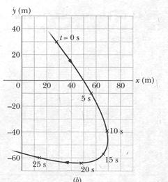
(b) Graph the rabbit's path for  to
to  s.
s.
Solution: We can repeat part (a) for several values of and then plot the results. Figure 4-36 shows the plots for five values of and the path connecting them. We can also use a graphing calculator to make a. parametric graph; that is, we would have the calculator plot у versus x, where these coordinates are given by Eqs. 4-5 and 4-6 as functions of time .
4-3 Average Velocity and Instantaneous Velocity
If a particle moves through a displacement in a time interval  , then its average velocity
  is
is
 Or
Or  (4-8)
(4-8)
This tells us the direction of must be the same as that of the displacement . Using Eq. 4-4, we can write Eq. 4-8 in vector components as
 (4-9)
(4-9)
For example, if the particle in Sample Problem 4-1 moves from its initial position to its later position in 2.0 s, then its average velocity during that move is
When we speak of the velocity of a particle, we usually mean the particle's instantaneous velocity  at some instant. This is the value that approaches in the limit as we shrink the time interval to 0 about that instant. Using the language of calculus, we may write as the derivative
 (4-10)
Figure 4-4 shows the path of a particle that is restricted to the  plane. As the particle travels to the right along the curve, its position vector sweeps to the right. During time interval , the position vector changes from to , and the particle's displacement is .
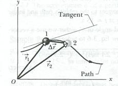 Fig. 4-4
|
To find the instantaneous velocity of the particle at, say, instant  (when the particle is at position 1), we shrink interval to 0 about . Three things happen as we do so: (1) Position vector in Fig. 4-4 moves toward so that shrinks toward zero. (2) The direction of
  (thus of ) approaches the direction of the tangent line to the particle's path at position 1. (3) The average velocity approaches the instantaneous velocity at .
In the limit as  , we have
  and, most important here, takes on the direction of the tangent line. Thus, has that direction as well:
► The direction of the instantaneous velocity of a particle is always tangent to the particle's path at the particle's position.
The result is the same in three dimensions: is always tangent to the particle's path.
To write Eq. 4-10 in unit-vector form, we substitute for from Eq. 4-1:
 .
.
This equation can be simplified somewhat by writing it as
 (4-11)
where the scalar components of are
 (4-12)
For example,  is the scalar component of along the axis. Thus, we can find the scalar components of by differentiating the scalar components of .
|
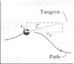
Figure 4-5 shows a velocity vector and its scalar x and у components. Note that is tangent to the particle's path at the particle's position. Caution: When a position vector is drawn, it is an arrow that extends from one point (a "here") to another point (a "there"). However, when a velocity vector is drawn as in Fig. 4-5, it does not extend from one point to another. Rather, it shows the instantaneous direction of travel of a particle located at the tail, and its length (representing the velocity magnitude) can be drawn to any scale.
 Sample Problem 4-3
For the rabbit in Sample Problem 4-2, find the velocity at time s, in unit-vector notation and as a magnitude and an angle.
Solution There are two Key Ideas here: (1) We can find the rabbit's velocity by first finding the velocity components. (2) We can find those components by taking derivatives of the components of the rabbit's position vector. Applying the first of Eqs. 4-12 to Eq. 4-5, we find the x component of to be
 (4-13)
At s, this gives  m/s.
m/s.
Similarly, applying the second of Eqs. 4-12 to Eq. 4-6, we find that the component is
At s, this gives  m/s.
m/s.
Equation 4-11 then yields
 (Answer)
which is shown in Fig. 4-6, tangent to the rabbit's path and in the direction the rabbit is running at s.
To get the magnitude and angle of , either we use a vector-capable calculator or we follow Eq. 3-6 to write
 m/s(Answer)
and  (Answer)
(Although 50° has the same tangent as -130°, inspection of the signs of the velocity components indicates that the desired angle is in the third quadrant, given by 50° - 180° = -130°.)
Date: 2015-01-12; view: 1406
| <== previous page | | | next page ==> |
| Acceleration | | | Average Acceleration and Instantaneous Acceleration |