The Domestic Mode of Production: Intensification of Production

Clearly the domestic mode of production can only be "a disarray lurking in the background," always present and never happening. It never really happens that the household by itself manages the econo­my, for by itself the domestic stranglehold on production could only arrange for the expiration of society. Almost every family living solely by its own means sooner or later discovers it has not the means to live. And while the household is thus periodically failing to provision itself, it makes no provision (surplus) either for a public economy: for the support of social institutions beyond the family or of collective activi­ties such as warfare, ceremony, or the construction of large technical apparatus—perhaps just as urgent for survival as the daily food sup­ply. Besides, the inherent underproduction and underpopulation posed by the DMP can easily condemn the community to the role of victim in the political arena. The economic defects of the domestic system are overcome, or else the society is overcome. The total empirical process of production is organized then as a hierarchy of contradictions. At base, and internal to the domestic system, is a primitive opposition between "the relations" and "the forces": domestic control becomes an impediment to development of the productive means. But this contradiction is reduced by imposing upon it another: between the household economy and the society at large, the domestic system and the greater institutions in which it is inscribed. Kinship, chieftainship, even the ritual order, whatever else they .may be, appear in the primitive societies as economic forces. The grand strategy of economic intensification enlists social structures beyond the family and cultural superstructures beyond the productive practice. In the event, the final material product of this hierarchy of contradictions, if still below the technological capacity, is above the domestic propensity.¹

The foregoing announces the overall theoretical line of our inquiry, the perspectives opened up by analysis of the DMP. At the same time, it suggests the course of further discussion: the play of kinship and politics on production. But to avoid a sustained discourse on generali­ties, to give some promise of applicability and verification, it is neces­sary first to attempt some measure of the impact of concrete social systems upon domestic production.

On a Method for Investigating the Social Inflection of Domestic Production

Given a system of household production for use, theory says that the intensity of labor per worker will increase in direct relation to the domestic ratio of consumers to workers (Chayanov's rule).²

1. The determination of the main organization of production at an infrastructural level of kinship is one way of facing the dilemma presented by primitive societies to Marxist analyses, namely, between the decisive role accorded by theory to the economic base and the fact that the dominant economic relations are in quality superstruct.ural, e.g., kinship relations (see Godelier, 1966;Terray, 1969). The scheme of the preceding paragraphs might be read as a transposition of the infrastructure-superstructure dis­tinction from different types of institutional order (economy, kinship) to different orders of kinship (household versus lineage, clan). In truth, however, the present problematique was not directly framed to meet this dilemma.

2. The same can be phrased also as an inverse relation between intensity and the proportion for workers, a formulation used earlier and to which we return presently.

The great­er the relative number of consumers, the more each producer (on average) will have to work to provide an acceptable per capita output for the household as a whole. Fact, however, has already suggested certain violations of the rule, if only because domestic groups with relatively few workers are especially liable to falter. In these house­holds, labor intensity falls below the theoretical expectation. Yet more important—because it accounts for some of the domestic default, or at least for its acceptability—the real and overall social structure of the community does not for its own part envision a Chayanov slope of intensity, if only because kin and political relations between households, and the interest in others' welfare these relations entail, must impel production above the norm in certain houses in a position to do so. That is to say, a social system has a specific structure and inflection of household labor intensity, deviating in a characteristic way and extent from the Chayanov line of normal intensity.

I offer two extended illustrations, from two quite different societies, to suggest that the Chayanov deviation can be depicted graphically and calculated numerically. In principle, with a few statistical data not difficult to collect in the field, it should be possible to construct an intensity profile for the community of households, a profile that indicates notably the amount and distribution of surplus labor. In other words, by the variation in domestic production, it should be possible to determine the economic coefficient of a given social sys­tem.

The first example returns to Thayer Scudder's study of cereal prod­uction in the Valley Tonga village of Mazulu. This study was consid­ered earlier in connection with domestic differences in subsistence production (Chapter 2). Table 3.1 presents the Mazulu materials in fuller form and in a different arrangement now including the number of consumers and gardeners by household and the domestic indices of labor composition (consumers/gardeners) and labor intensity (acres/gardener). The Mazulu data offer no direct measure of labor intensity, such as the actual hours people work; intensity has to be understood indirectly by the surface cultivated per worker. Imme­diately an error of some unknown degree is introduced, since the effort expended/acre is probably not the same for all gardeners. More­over, in the attempt to account for the fractional dietary requirements and labor contributions of different sex and age classes, some esti­mates had to be made, as a detailed census is not available and the population breakdown in Scudder's production tables (1962, Appen­dix B) is not entirely specific. Insofar as possible, I apply the following rough and apparently reasonable formula for assessing consumption requirements: taking the adult male as standard (1.00), preadolescent children are computed as 0.50 consumers and adult women as 0.80 consumers.³ (This is why the consumer column yields a figure less than the total household size, and usually not a whole number.) Finally, adjustments had to be made for calculation of the domestic labor force. A few very small plots appearing in Scudder's table were evidently the work of quite young persons; probably these were train­ing plots in the charge of younger adolescents. Gardeners listed by Scudder as cultivating less than 0.50 acres and belonging to the youngest generation of the family are thus counted as 0.50 workers.

3. All persons indicated in Scudder's table as "unmarried people for whom the wife must cook", and who were not further tabulated as gardeners, were counted as preado-lescent children. Probably some dependent elders have thus slipped in as 0.50 consum­ers.

Table 3.1. Household variations in intensity of labor: Mazulu Village, Valley Tonga, 1956-57 (after Scudder, 1962, pp. 258-261)

♦In families D and L, the head of the house was absent in European employ during the entire period. He is not calculated in the household's figures, although the money he brings back to the village will presumably contribute to the family's subsistence.

t The head of the house, K, worked part time in European employ. He also cultivated and figures in the computations for his household.

Manifestly, I must insist on the illustrative character of the Mazulu example. In addition to the several errors potentially introduced by one's own manipulations, the very small numbers involved—there are only 20 households in the community—cannot inspire a grand statis­tical confidence. But as the aim is merely to suggest a feasibility and not to prove a point, these several deficiencies, while surely regretta­ble, do not seem fatal.⁴

4. Besides incertainties in the data, there are external complications, some of which are indicated in footnotes to Table 3.1. One, however, must be considered in greater detail There is a modest amount of cash cropping in Mazulu, mainly of tobacco, with the proceeds invested principally in animal stock. The effects upon the domestic prod­uction of cereals are not altogether clear, but the figures on hand probably have not been seriously deformed by crop sales. The total volume of produce sale is quite limited; of subsistence crops in particular, insignificant. At the time of study, Scudder writes, "most valley Tonga were essentially subsistence cultivators who rarely sell a guinea's worth of produce per annum" (1962, p. 89). Nor did cash cropping appear an alterna­tive to subsistence gardening, that is, as a means of food purchase, so capable of direct interference in cereal cultivation. Finally, in such cases of simple commodity produc­tion, it must be considered whether trade actually removes the exchangeable food sur­plus from internal community circulation. It happens that those Tongan farmers who convert produce into animal stock are precisely the ones most subject to imperious re­quests from relatives at times of food shortage—for animals constitute a reserve that may be again sold for grain (pp. 89 f, 179-180; Colson, 1960, p. 38 0-

What then do the Mazulu materials illustrate? For one, that Chayanov's rule holds—in a general way. That the rule holds in general, although not in detail, is evident by inspection of the final columns of Table 3.1. The acreage cultivated/gardener mounts in rough relation to the domestic index of consumers/gardener. A proce­dure like Chayanov's own would show the same, with a little more exactness. Following Chayanov's methods, Table 3.2 groups the vari­ation in acreage/worker by regular intervals of the consumer/worker index:

Table 3.2. Household variations in acreage/gardener: Mazulu*

*One further complication of the Mazulu data: in richer households able to provide beer for outside workers, some of the labor expended does not come immediately from the domestic group in question. On one hand, then, the figures for acreage cultivated/worker do not do justice to the actual force of the Chayanov principle-richer houses are working less than indicated, poorer more. On the other hand, some portion of the beer so provided may represent the congealed labor of the supplying household, so that over the longer run the slope of intensity /worker is closer again to the data reported. Clearly subtle corrections aie necessary, or else direct estimates of hours worked per gardener-both beyond the prerogatives given by the present data.

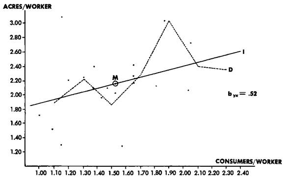
The results are fairly comparable to those Chayanov and his co­workers found for peasant Russia. Yet the Mazulu table also betrays the rule. Clearly the relation between labor intensity and the house­hold ratio of workers is neither consistent nor proportionate over the entire range. Individual houses deviate more or less radically, but not altogether randomly, from the general trend. And the trend itself does not develop evenly: it takes on an irregular curvature, a specific pattern of rise and fall.

All this trend and variation can be plotted on a single graph. The scatter of points in Figure 3.1 represents the distribution of household differences in labor intensity. Each house is fixed relative to the hori­zontal (X) axis by its ratio of consumers/gardener, and along the vertical (Y) axis by the acreage cultivated/gardener (cf. Table 3.1). A midpoint to this variation, a kind of average household, can be de­termined at X = 1.52 (c/w), Y - 2.16 (a/w).The overall average tendency of household differences in intensity is then calculable by deviations from this mean, that is, as a linear regression computed according to standard formula.⁵

5.6xy= t (xy)/ 2 (x²), where x = the deviation of each unit from the x mean (c/w mean), y the deviation from the y (a/w) mean. Given the limited and scattered distribution of household differences, it should be stressed that the regression in the Mazulu case (and in subsequent cases treated) has little predictive or inductive value. It has been adopted here simply as a description of the main drift in the variations.

The result for Mazulu, the real intensity slope of the community, amounts to an increase of 0.52 acres/ worker (Y) for each additional 1.00 in the ratio of consumers to workers (X). But artificially so. The broken line (D) of Figure 3.1 seeks out the truer course of variation, the important propensity to depart from a linear relation between intensity and composition. This line, the real intensity curve, is constructed after the mean intensities (columnar means) of 0,20 intervals in the consumers/worker ratio. Note that the curve would have taken a somewhat different path if plotted from the value? of Table 3.2. But with so few cases at hand, 20 households, it is difficult to say which version is more valid. Statistical intuition might hold that with more instances the Mazulu curve would be sigmoidal (an \J^ curve), or perhaps concave upward to the right in exponential fashion. Both of these patterns, and others besides, occur in Chayanov's own tables. What seems more impor­tant, however, and consistent with accomplished understandings, is that the variation in labor intensity increases toward both extremes of the c/w range, disturbing or even reversing the more regular incline of the medial section. For at the extremes of household composition, Chayanov's rule becomes vulnerable to contradiction. On one side are households weak in manpower and subject to one or another crippling malchance. (Household J in the Mazulu series, represented by the point furthest right, is an instance in question: a woman widowed at the beginning of the cultivation period and left to support three prea-dolescent children.) On the other side, the decline of the intensity curve to the left is arrested at some moment because certain domestic groups well endowed in workers are functioning beyond their own necessity. From that point of view (that is, of their own customary requirements), they are working at surplus intensities.

Figure 3.7. Mazulu: Trend and Variation in Household Labor Intensity

But the surplus output is not exactly indicated by the foregoing procedure. For this it is necessary to construct a slope of normal intensity, drawn as much from theory as from reality: a slope de­scribing the variation in labor that would be required to supply each household the customary livelihood, supposing each were left to provision itself. It is necessary, in other words, to project the domestic mode of production as if unimpeded by the larger structures of socie­ty. The performance to which the DMP as such is disposed, this line of normal intensity might also then be deemed the true Chayanov slope, for it represents the most rigorous statement of the Chayanov rule. Insofar as it is predicated on production to a definite and custom­ary goal, Chayanov's rule does not admit just any proportionate relation between intensity and relative working capacity. In principle it stipulates strictly the slope of this relation: the domestic intensity of labor must increase by a factor of the customary consumption requirement for every increase of 1.00 in the domestic ratio of con­sumers to workers. Only in that event will the same (normal) output per capita be achieved by each household, regardless of its particular composition. This, then, is the intensity function that conforms to the theory of domestic production—as the deviation from it in actual practice conforms to the character of the larger society.

How do we determine the true Chayanov slope for Mazulu? Ac­cording to Scudder, 1.00 acres under cultivation per capita should yield an acceptable subsistence. But "per capita" here applies indis­criminately to men, women and children. As by our earlier computa­tion the village population of 123 reduces to 86.20 full consumers (adult male standard), each consumer of account will demand 1.43 acres for a normal subsistence. The true Chayanov slope is therefore a straight line departing from the origin of both dimensions and rising 1.43 acres/gardener for every increase of 1.00 in the domestic ratio of consumers to workers.

Before proceeding to measure real deviations from this slope, some decision has to be taken between alternative formulations of the Chay­anov rule, as this has a practical bearing on the representation of normal intensity. Most of the preceding discussion has been content to refer to intensity rising with the relative number of consumers. Yet the law of Chayanov is just as well expressed as an inverse relation between domestic intensity and the relative number of producers; that is, the fewer the producers to consumers, the more each will have to work. Logically, the two propositions are symmetrical. But sociologi­cally, perhaps not. The first seems to better express the operative constraints, the burdens imposed upon able-bodied producers by the dependents they must feed. Probably that is why Chayanov in effect preferred the direct formulation, and I shall continue to do so.⁶

6. For a diagrammatic indication of Chayanov's rule formulated as an inverse relation, see the interesting analysis of the covariation between domestic labor force and preferred intensities of labor among Indian farm families presented in Clark and Haswell, 1964, p. 116.

In Figure 3.2, then, the Chayanov line (C) rises upward to the right, intensity increasing with the relative number of consumers by the calculated factor of 1.43 a/w per 1.00 c/w. The line threads its way through a scatter of points. Once more these stand for the de facto household differences in labor intensity. But in juxtaposition to the true Chayanov slope, their meaning is transformed: They tell now of the modification imparted to domestic production by the greater organization of society.This modification is summarized also by the deviation of the real intensity slope (I) from the Chayanov, insofar as the former—0.52 a/w for each 1.00 c/wfrom the means of intensity and composition—represents a reduction of household production differences to their main drift. The positioning of these lines, their manner of intersection within the range of known domestic variations, makes a profile specific to that community of the societal transforma­tion of domestic production (Figure 3.2).

The Mazulu profile can be sharpened and certain of its configura­tions measured. The empirical production slope (I) passes upward to the left of the Chayanov intensity (C), to an important extent because certain households, among them many with favorable manpower re­sources, are cultivating above their own requirements. They are work­ing at surplus intensities, not simply for their own use, because they are included in a social system of production, not simply a domestic system. They contribute to the larger system surplus domestic labor. Eight of the 20 Mazulu producing groups are so engaged in extraor­dinary efforts, as shown in Table 3.3. Their own average manpower structure is 1.36 consumers/worker, and their mean intensity 2.40 acres/gardener. Let us mark this point of mean surplus labor, point S, on the Mazulu profile (Figure 3.2). Its coordinates express the Mazulu strategy of economic intensification. The vertical distance of S over the slope of normal intensity (segment ES ) constitutes the mean impulse to surplus labor among productive houses: 0.46 acres/ worker or 23.60 percent (as normal intensity at 1.36 c/wis 1.94 a/w). There are 20.50 effective producers in these houses, or 35.60 of the village labor force. Thus 40 percent of the domestic producing groups, comprising 35.60 percent of the working force, are functioning at a mean of 23.60 percent above the normal intensity of labor. So for the Y -value of S.

Figure 3.2. Mazulu: Empirical and Chayanov Slopes of Labor Intensity

Table 3.3. Normal and empirical variations in domestic labor intensity: Mazulu

The X coordinate of the surplus impulse (S) will by its relation to mean household composition (M) provide an indication of how the intensification tendency is distributed in the community (Figure 3.2). The further S falls to the left of the mean composition (X = 1.52 c/w), the more surplus labor is a function of higher proportions of workers in the domestic group. A position of S nearer the mean, however, indicates a more general participation in surplus labor: further still to the right, S would imply an unusual economic activity in house­holds of lesser labor capacity. For Mazulu, the mean surplus impulse (S) is clearly left of the village mean. Six of the eight houses functioning at surplus intensities are below average in their ratios of consum­ers/worker. For all eight, the mean composition is lower than the community average by 0.16 c/w or 10.50 percent.

Finally it is possible from the materials on hand (Tables 3.1 and 3.3) to compute the contribution of surplus (domestic) labor to the total village product. This is done by first calculating the sum of surplus acreage in the several houses producing above normal intensity (num­ber of workers multiplied by the rate of surplus labor for the eight relevant cases). The output thus attributable to surplus labor is 9.21 acres. The total cultivations of Mazulu amount to 120.24 acres. Hence, 7.67 percent of the total village output is the product of surplus labor.

It has to be emphasized that "surplus labor" applies strictly to the domestic groups, and that it is "surplus" in relation to their normal consumption quota. Mazulu village as a whole does not show a sur­plus expenditure of labor. It is testimony rather to the character and relative ineffectiveness of the existing social strategy that the total acreage cultivated falls slightly below village requirements. (Thus at the point of mean household composition [1.52 c/w],the empirical inflection of production [/] passes under the true Chayanov slope [C].) A nonproductive class could not live on the output of the Mazu­lu villagers—at least not without substantial contradiction and poten­tial conflict.

The mathematical reason for village underproduction is obvious. If some domestic groups are functioning above normal intensity, others are working below, to the extent that village output is on balance slightly negative. But this distribution is not accidental. On the con­trary, the entire production profile should be understood as an inte­grated social system in its projection of normal domestic intensity as well as its empirical labor slope, in its dimension of domestic under­production as well as domestic surplus. The subintensive output of some houses is not independent of the surplus labor of others. True that (as far as our information goes) household economic failures seem attributable to circumstances external to the organization of production: illness, death, European influence. Yet it would be mis­leading to contemplate these failures in isolation from the successes, as if certain families simply proved unable to make it for reasons entirely their own. Some may not have made it precisely because it was clear in advance they could depend on others. And even the underproduction due to unforeseen circumstances is acceptable to society, these vulnerable households tolerable, by virtue of a surplus intensity elsewhere, which in a sense had anticipated in its own dy­namic a certain social incidence of domestic tragedy. In an intensity profile such as Figure 3.3, we have to deal with an interrelated distrib­ution of household economic variations—that is, with a social system of domestic production.

The Kapauku of western New Guinea have another system, very different in its pattern, much more pronounced in its strategy of intensification. But then, Kapauku is another politicalsystem, capable of harnessing domestic economic efforts to the accumulation of ex­changeable products, pigs and sweet potatoes primarily, whose sale and distribution are main tactics of an open competition for status (Pospisil, 1963).

Sweet potato cultivation is the key sector of production. The Ka­pauku to a very large extent, and their pigs to a lesser extent, live by sweet potato. It accounts for over 90 percent of the agricultural land use and seven-eighths of the agricultural labor. Yet the domestic differences in sweet potato production are extraordinary: a tenfold range of variation in output/household as recorded by Pospisil for the 16 houses of Botukebo village over an eight-month period (Table 3.4).

Again for Kapauku we know the intensity of labor only by its product. The intensity column of Table 3.4 is presented as kilograms of sweet potato produced per worker—probably introducing an error analogous to the corresponding Mazulu figures, insofar as different workers expend unequal efforts per unit weight of output. I have taken the liberty, moreover, of revising the ethnographer's household consumer counts, bringing them closer in line with other Melanesian societies by assessing adult women at 0.80 of the adult male require­ment, rather than the 0.60 Pospisil had computed from a brief dietary study. (For the other members of the household, children were fig­ured at 0.50 consumers, adolescents at 1.00 and elders of both sexes at 0.80.) Adolescents were calculated at 0.50 workers, following the ethnographer's usage.

Domestic differences in labor intensity compose a very distinctive pattern. No clear Chayanov trend is evident on inspection of Table 3.4. But the apparent irregularity polarizes, or, rather, resolves itself into two regularities once the household variations are plotted in graph (Figure 3.3). Everything appears as if the Kapauku village were divided into two populations, each adhering singularly to its own economic inclination in one case, something of a Chayanov trend, intensity increasing with the relative number of consumers, yet in the other "population" just the reverse. And not only are houses of the latter series industrious in proportion to their working capacity, the group as a whole stands at a distinctly higher level than the house­holds of the first series. But then the Kapauku have a big-man system of the Classic Melanesian type (seebelow,"The Economic Intensity of the Social Order"), a political organization that typically polarizes people's relations to the productive process: grouping on one side the big-men or would-be big-men and their followers, whose production they are able to galvanize, and on the other side those content to praise and live off the ambition of others.⁷

7. Subject to the caveat, actually realized in the Botukebo case, where the big-man's production is not extraordinary, that a leader who has successfully piled up credits and followers may eventually slacken his own particular efforts.

The idea seems worth a prediction: that this bifurcate, "fish-tail" distribution of domestic labor intensity will be found generally in the Melanesian big-man systems.

Table 3.4. Household variation in sweet potato cultivation: Botukebo village, Kapauku (New Guinea), 1955 (after Pospisil, 1963)

*See text for discussion of "revised" consumer estimates.

t Calculated at adults (9 and d) = 1.00 worker, adolescents and elders of both sexes at 0.50 worker.

Although not evident to inspection, a light Chayanov trend does actually inhere in the scatter of household intensity variations. It has to be picked up mathematically (again as a linear regression of devia­tions from the means). On balance, the slope of domestic labor intensi­ty moves upward to the right at the rate of 1,007 kilograms of sweet potato/gardener for each increase (from the mean) of 1.00 in the consumers/gardener ratio. Considered by their respective standard deviations, however, this Kapauku inflection is flatter than the Mazulu empirical slope. In z-units, by* = 0.62 for Mazulu, 0.28 for Botukebo.) Yet more interesting, the Kapauku real inflection stands in an entirely different relation to its slope of normal intensity (Figure 3.4).

I have plotted the slope of normal intensity (the true Chayanov cline) from Pospisil's brief dietary study covering 20 people over six days. The average adult male ration was 2.89 kilograms of sweet potatoes/day—693.60 kilograms, then, for an eight-month period matching the duration of the production study. An inflection of 694 kilograms/worker for each 1.00 in c/w passes substantially underneath the empirical intensity slope, indeed, it does not intersect the latter through the range of real variations in domestic production. The profile is altogether different from Mazulu, and as different in its indicative measures.⁸

8. A theoretical argument can be made for inclusion in the domestic quotas of consumption, hence in the slope of normal intensity, an extra amount of sweet potato equivalent to the feed that would be needed to supply a normal per capita pork ration. Apart, however, from arguments also possible to the contrary, the published data do not readily lend themselves to this calculation.

Figure 3.3. Botukebo Village, Kapauku: Domestic Variations in Labor Intensity (1955)

Figure 3A. Botukebo, Kapauku: Social Deviation of Labor Intensity from the Chayanov Slope

Nine of the 16 Botukebo households are operating at surplus inten­sities (Table 3.5). These nine houses include 61.50 gardeners, or 59 percent of the total working force. Their average composition is 1.40 consumers/gardener, their mean labor intensity, 1,731 kilograms/gar­dener. Hence the point of mean surplus labor, S_t falls slightly to the right of the average household composition—by two percent of the c/w ratio. In fact, six of the nine houses are below average compos­ition, but not dramatically so. The impulse to surplus labor thus appears more generally distributed in Kapauku than in Mazulu. At the same time, the strength of this impulse is definitely superior. As expressed by the Y coordinate of S, the mean tendency of surplus intensity, at 1,731 kilograms/worker, is 971 kilograms above the nor­mal tendency (segment SE). In other words, 69 percent of the Kapau-ku domestic units, comprising 59 percent of the labor force, are working at an average of 82 percent above normal intensity.

Table 3.5. Botukebo, Kapauku: Domestic variation in relation to normal intensity of labor

The collective surplus labor of these Kapauku units accounts for 47,109 kilograms of sweet potato. Botukebo total village output is 133,172 kilograms. Thus, 35.37 percent of the social product is the contribution of surplus domestic labor. Taken in comparison with Mazulu (7.67 percent), this figure makes us aware of something here­tofore left out of account: the customary household structure is also part of the society's intensification strategy. Botukebo's advantage over Mazulu does not consist solely in a higher rate or more general distribution of surplus labor. Botukebo houses have on average more than twice as many workers, so multiply by that difference their superiority in rate of intensity.

Finally, as the Kapauku intensity profile shows, the effect of sur­plus labor is to displace real domestic output upward by a sizable amount over the normal. At mean household composition, the empiri­cal inflection of intensity is 309 kilograms/worker (29 percent) higher than the Chayanov slope (segment M-M'of Figure 3.4). In terms of the people's own consumption requirements (pigs excluded), Botuke­bo village as a whole has a surplus output.⁹

9. Pigs included, village production still surpassed the collective subsistence norm (Pospisil, 1963, p. 3940-

Table 3.6 summarizes the differences in production intensity be­tween Mazulu and Botukebo. These differences are the measure of two different social organizations of domestic production.

Table 3.6. Indices of domestic production: Mazulu and Botukebo

*Concerns households working at surplus intensity.

But clearly the task of research is not finished by the drawing of an intensity profile; it is only thus posed. Before us stretches a work of difficulty and complexity matched only by its promise of an anthro­pological economics, and consisting not merely in the accumulation of production profiles, but of their interpretation in social terms. For Mazulu and Botukebo this interpretation would dwell on political differences—on the contrast between the big-man system of the Ka­pauku and traditional political institutions described by the ethnographer of Tonga as "embryonic," "largely egalitarian" and generally disengaged from the domestic economy (Colson, 1960, pp. 1610- It remains to specify such relations between political form and economic intensification; and also, the less dramatic economic impact of the kinship system, almost imperceptible for its prosaic, everyday charac­ter but perhaps not less powerful in the determination of everyday production.

Date: 2014-12-21; view: 1725