CATEGORIES:
BiologyChemistryConstructionCultureEcologyEconomyElectronicsFinanceGeographyHistoryInformaticsLawMathematicsMechanicsMedicineOtherPedagogyPhilosophyPhysicsPolicyPsychologySociologySportTourism
The graph in Figure 3.3.
a single absorbing state: E\ = (all-D) and E2 = {all-Q|. We need to find the least resistant path from £i to £2, and also from E2 to £]. Consider the first case. If the process is in the all-D state, and exactly one player makes an error (plays Q), then we obtain a state such as the following: DDDQ DDDD ■n the next period, both players will choose D as a best reply to any sample of size two; hence, if there are no further errors, the process will revert back (after four periods) to the state, all-D. Sl|ppose now that two players simultaneously make an error, so that We obtain a state of the following form:
Figure 3.5. The resistances of the two rooted trees in the typewriter game with learning parameters m = 4, s = 2. Again, the unique best reply to every subset of size two is D. Hence, if there are no more errors, the process drifts back to the all-D state. Suppose however that two errors occur in succession in the same population: DDQQ DDDD From this state, there is a positive probability (though not a certainty) of transiting to the all-Q state with no further errors. The most probable transition from all-D to the above state occurs in two steps, each step having probability on the order of e. Thus the resistance to moving from Ei to £2 is Г]2 = 2. On the other hand, if we begin in E2 = {all-Q}, a single choice of D suffices for the process to evolve (with no further errors) to the all-D state. Hence, Г21 =1. The two rooted trees for this example are quite trivial: each contains one edge, as shown in Figure 3.5. The tree with least resistance is the one that points from vertex 2 (all-Q) to vertex 1 (all-D). From the theorem, we therefore conclude that the unique stochastically stable state is all-D. In other words, when e is small, the long-run probability of being in this state is far higher than that of being in any other state.
To get a feel for the extent to which the probability accumulates on all-D as a function of e, we may simulate the process by Monte Carlo methods. (This is only practical when the state space is small, as in the present example.) The results for selected values of e are summarized in Table 3.1. Note that, even with a sizable error rate (say, e = .20), the
expected proportion of D-players is over 80 percent. This illustrates the point that the stationary distribution can put high probability on the stochastically stable states even when e is fairly large. The virtue of theorem 3.1 is that it tells us where the long-run probability of the learning process is concentrated when we lack a precise estimate of e, but know that it is "small." If we did know e precisely, we could (in theory) compute the actual distribution pe. However, it would be very cumbersome to solve the stationarity equations (3.7) directly, because of the unwieldy size of the state space. Fortunately, there is a second way of computing pr that yields analytically tractable results in certain situations. Like the computation of the stochastic potential function, the computation of д' is based on the notion of rooted trees. Unlike the former case, however, these trees must be constructed on the whole state space Z. Hence the approach is analytically useful only in certain special cases. Let P be any irreducible Markov process defined on a finite state space Z. (Note that P does not have to be a regular perturbed process.) Consider a directed graph having vertex set Z. The edges of this graph form a z-tree (for some particular z 6 Z) if it consists of |Z| - 1 edges and from every vertex z' ф z there is a unique directed path from z! to z. Directed
edges can be represented by ordered pairs of vertices (2. z'), and we can represent a z-tree T as a subset of ordered pairs. Let T: be the family of all z-trees. Define the likelihood of z-tree T 6 T: to be P(T)= П p The following result is proved in the Appendix. lemma 3.1 (Freidlin and Wentzell, 1984). Let P be an irreducible Markov process on a finite state space Z. Its stationary distribution ц has the property that the probability p(z) of each state z is proportional to the sum of the likelihoods of its z-trees, that is, tx(z) = v(z)/ Y^ "(«'). where v(z) = ^ P(T). weZ TeT: To illustrate the difference between this result and theorem 3.1, consider a Markov process with seven states Z = [a. b. c, d. e. f. g} and the transition probabilities shown in Figure 3.6. (It is understood that the probability of staying in a given state is one minus the total probability of leaving it in each period.) This process has an essentially linear structure, that is, transitions can occur only to a "neighboring" state. This means that for each state z, there is a unique z-tree having nonzero probability. For example* the unique c-tree consists of the directed edges a -*■ b, b -*■ c, d -* c> e -> d, f e, g /. Lemma 3.1 tells us that the likelihood of a z- tree is proportional to the probability of z in the stationary distribution. It is a simple matter to compute the likelihood of each such tree—the tree's likelihood is just the product of the probabilities on its edges. A State: a b с d e f g Relative probability: £2/24 5г3/9 5e>/12 5 c2/24 e2/24 e/48 e/32 Note that this estimate is exact for each e > 0; it is not a limiting result as e approaches zero. When e is small, however, we can see immediately that states / and g will be much more likely than any of the other states. We will now show how theorem 3.1 leads to the same conclusion by a different route. Let P denote the transition matrix of the process as a function of e. First, we observe that the unperturbed process P° has exactly two recurrent classes: Ei = (л|, and £2 = {/.#)• Then we compute the resistances from E\ to £2, and vice versa (see Figure 3.7). On one hand, the least resistant path (among all feasible paths) from £1 to £2 has probability Юе x 1/4 x 1/2 x 1/10 x 1/2 x 1/2 = e/32. Since this involves e to the first power, the resistance is Г12 = 1- On the other hand, the least resistant path from E2 to E\ involves e to the second power; hence r21 = 2. The graph from which we compute the stochastic potential is therefore quite trivial: it consists of two vertices and two directed edges. The least resistant Ei-tree consists of the single edge £2 —► £], whose resistance is 2. The least resistant Ет-tree consists of the single edge £1 E2, whose resistance is 1. Thus the stochastic Potential of £t equals 2, and the stochastic potential of E2 equals 1. It follows from theorem 3.1 that E2 is stochastically stable, which is exactly what the previous calculation showed in a more detailed way.
While lemma 3 .1 gives a more precise estimate of the stationary distribution, both approaches can be used to compute the stochastically stable In subsequent chapters, we shall examine the implications of these ideas for various classes of games. The theory provides sharp predictions about the equilibrium (and disequilibrium) configurations that are selected by simple learning rules. Moreover, it shows how key solution concepts in the game theory literature that are traditionally justified by high-rationality arguments—including the Nash bargaining solution in bargaining games (see Chapter 8), and efficient coordination equilibria in pure coordination games (see Chapter 9)—can emerge in low- rationality environments as well. It should be emphasized, however, that this approach is very general and can be used to study a variety of dynamic processes, not just the adaptive playing of games. 3.5 The Neighborhood Segregation Model To illustrate this point, consider the neighborhood segregation model discussed in Chapter 1. Individuals are located at n possible positions around a circle, and they are of two types: A and B. A state z of the system is an assignment of A or В to each position. To avoid trivialities we assume that there are at least two individuals of each type. Individuals are discontent if both immediate neighbors are of the opposite type; otherwise they are content. In each period, one pair of individuals is selected at random, where all pairs are equally likely to be chosen. Consider such a pair of individuals, say / and j. The probability that they trade depends on their prospective gains from trade. Let us assume that every trade involves moving costs. Thus there can be positive gains from trade only if the partners are of opposite types and at least one of them (say i) was discontent before and is content afterwards. This means that before the trade i was surrounded by people of the opposite type, so in fact both i and j are content afterwards. (We shall assume that if j was content before and after, i can compensate j for his moving costs and still leave both better off.) Such Pareto improving trades are said to be advantageous; all other trades are disadvantageous. Assume that each advantageous trade occurs with high probability, and that each disadvantageous trade occurs with a low probability that decreases exponentially with the partners' net loss in utility. Specifically, let us suppose that there exist real numbers 0 < a < b < с such that the probability of a disadvantageous trade is e" if one partner's increase in contentment is offset by the other's decrease in contentment (so the net losses involve only moving costs), the probability is e1' if both partners were content before and one is discontent after, and it is ec if both were content before and both are discontent after. (These are the only possibilities.) Advantageous trades, by contrast, occur with probabilities that approach one as e —► 0; beyond this we need not specify the probabilities exactly. The resulting Markov process P' is irreducible for every e > 0, and satisfies conditions (3.11) and (3.12). A state of the unperturbed process P° is absorbing if each person is located next to somebody of his or her own type. A state is segregated if the As form one contiguous group, and the Bs form the complementary group. In Chapter 1 we asserted that the segregated states are the only stochastically stable states of the perturbed process P. We shall now establish this fact using the theory described in the preceding section. The first step is to identify the recurrent communication classes of P°. These obviously include the absorbing states, which are singleton recurrent classes. To prove that these are the only recurrent classes, consider a state that is not absorbing. It contains at least one discontent individual, say i, who we may assume is of type A. Going clockwise around the circle, let i' be the next individual of type A. (Recall that there are at least two individuals of each type.) The individual just before /' must be of type B. Call this individual j. If i and j trade places, both will be content afterwards. In any given period there is a positive probability that this pair will in fact be drawn, and that they will trade. The resulting state has fewer discontent individuals. Continuing in this manner, we see that from any nonabsorbing state there is a positive probability of transiting to an absorbing state within a finite number of periods. Hence the absorbing states are the only recurrent states. Denote the set of absorbing states by Z°. For any two states z and z' inZ°, let r(z, z') denote the least resistance among all paths from z to z'. The stochastic potential of z e Z° is defined to be the resistance of the
minimum resistance z-tree on the set of nodes Z°. By theorem 3.1, the stochastically stable states are those with minimum stochastic potential. It therefore suffices to show that an absorbing state has minimum potential if and only if it is segregated. To prove this we proceed as follows: let Z° = Z' U Z"s where Zs is the set of segregated absorbing states and Z"s is the set of nonsegregated absorbing states. We claim that: (i) for every z e Z"s, every z-tree has at least one edge with resistance b or с (which are greater than a); and (ii) for every z e Zs, there exists a z-tree in which every edge has resistance exactly equal to a. Assume for the moment that (i) and (ii) have been established. In any z-tree there are exactly |Z"| - 1 edges, and the resistance of each edge is at least a. It follows from (i) and (ii) that the stochastic potential of every segregated state equals a\Z°\ - a, while the stochastic potential of every nonsegregated state is at least fl|Z(,| -2a + b, which is strictly larger. Theorem 3.1 therefore implies that the segregated states are precisely the stochastically stable states. To establish (i), let z e Z"s be a nonsegregated absorbing state. Given any z-tree T, there exists at least one edge in T that is directed from a segregated absorbing state 2s to a nonsegregated absorbing state zm. We claim that any such edge has a resistance of at least b. The reason is that any trade that breaks up a segregated state must create at least one discontent individual, hence the probability of such a trade is either e1' or ec (see Figure 3.8). Thus the resistance of the edge from z* to z"s must be at least b, which establishes (i). To establish (ii), let zeZsbea segregated absorbing state. From each state z' Ф z we shall construct a sequence of absorbing states 2' = zKz2................ 2* = 2 such that r(z/~l,zi) = a for I < j < k. Call this a 2'2-path. We shall carry out the construction so that the union of all of the directed edges on all of these paths forms a 2-tree. Since each edge has a resistance of a and the tree has |Z°| - 1 edges, the total resistance of the tree is a\ZQ\ - a as claimed in (ii). Suppose first that 2' is also segregated, that is, 2' consists of a single contiguous A-group and a complementary contiguous B-group. Label the positions on the circle 1.2..................... и in the clockwise sense. Let the first member of the A-group trade places with the first member of the B-group. Since both were content before and after, this trade has probability s". It also results in a new absorbing state, which shifts the A-group and the B-group by one position clockwise around the circle. Hence within n steps we can reach any absorbing state, and in particular we can reach 2. Thus we have constructed a sequence of absorbing states that leads from 2' to 2, where the resistance of each successive pair in the sequence equals a. Suppose alternatively that 2' is not segregated. Moving clockwise from position 1, let A denote the first complete group of contiguous As. Let В be the next group of Bs, and A' the next group of As. Since z' is absorbing, each of these groups contains at least two members. Let the first player in A trade places with the first player in B. Since both players were content before and after the trade, its probability equals e". This trade shifts group A one position clockwise and reduces by one the number of В players between A and A'. It either results in a new absorbing state, or else a single В player remains between A and A'. In the latter case this В player can then trade with the first player in group A, and this trade has zero resistance. The result is an absorbing state with fewer distinct groups of As and Bs. Repeat the process described in the preceding paragraph until all the As are contiguous and all the Bs are contiguous. Then continue as in the earlier part of the argument until we reach the target state 2. This construction yields a sequence of absorbing states that begins at 2' and ends at 2, where the resistance between each successive pair of states is л. The path contains no cycles because the number of distinct groups never increases; indeed with each transition one of the groups shrinks until it is eliminated. Thus the union of these paths forms a z-tree whose total resistance is a|Z°| - a. This concludes the proof that the stochastically stable states are precisely the segregated ones.6 Chapter 4 ADAPTIVE LEARNING IN SMALL GAMES IN THIS CHAPTER, we explore the properties of adaptive learning in two- person games, where each player has exactly two actions. Although this is a special case, it can be used to illustrate a wide variety of social and economic interactions. We begin by introducing the classical notion of risk dominance in 2 x 2 games, and then show that it coincides with the stochastically stable outcome under a variety of assumptions about the learning process. In larger games, however, the two concepts differ, as we shall show in Chapter 7. 4.1 Risk Dominance Consider a two-person game G with payoff matrix
G is a coordination game with pure strategy Nash equilibria (1, 1) and (2, 2) if and only if the payoffs satisfy the inequalities «11 > «21. fell > &12.«22 > «12.&22 > Ь21- (4-2) Equilibrium (1, 1) is risk dominant if (On - Л21)(Ьц - bu) > («22 - «12)(t>22 ~ &2l)- (4.3) Similarly, equilibrium (2, 2) is risk dominant if the reverse inequality holds (Harsanyi and Selten, 1988). If the inequality holds strictly, the corresponding equilibrium is strictly risk dominant.1 Risk dominance has a particularly simple interpretation when the game is symmetric. Consider the symmetric payoff matrix
Imagine that each player is uncertain about the action that the other player is going to take. If each has a flat prior (attaches a fifty-fifty probability to the intended action of the other), the expected payoff from playing action 1 is (a+c)/2, while the expected payoff from action 2 is (d + b)J2. An expected utility maximizer therefore chooses action 1 only if (а + с)/2 > (d + b)/2, that is, only if a - d > b - c. This is equivalent to saying that action 1 is risk dominant. In other words, when each player assigns equal odds to his or her opponent's playing action 1 or 2, both players will choose a risk-dominant action. In the more general case (4.1), we can motivate risk dominance as follows. Define the risk factor of equilibrium (/. i), where / = 1,2, to be the smallest probability p such that if one player believes the other player is going to play action i with probability strictly greater than p, then i is the unique optimal action to take.2 Consider, for example, equilibrium (2.2). For the row player, the smallest such p satisfies «п (1 ~p)+a\2p = «21(1 - p)+a22p, that is, p = (ЯЦ - я2,)/(яи - я12 - Я21 + я22). (4.5) For the column player, the smallest such p satisfies fend ~p) + b2\p = fei2(l -p) + Ьтгр. that is, p = (fen - bn)/(bu - b]2 - b2\ + М- (4.6) In general, let a = («и - «2i)/(«n - fl]2 - я21 + a22) and /3 = (fen - fen)/(fen - fen - fe2i + fe22). (4.7) chapter 4 The risk factor for equilibrium (2, 2) is therefore а л f), where in general x л у denotes the minimum of .y and y. Similarly, the risk factor for equilibrium (1, 1) is (1 - а) л (1 - f)). A risk-dominant equilibrium in a 2 x 2 game is an equilibrium whose risk factor is lowest. Thus equilibrium (1,1) is risk dominant if and only if а л(1-е) л (1-0). (4.8) Equilibrium (2, 2) is risk dominant if and only if the reverse inequality holds. A little algebraic manipulation shows that (4.8) is equivalent to (On - fl2l)(bll - bn) > («22 - «12)(&22 ~ bU)- (4.9) In other words, in a 2 x 2 game an equilibrium is risk dominant if and only if it maximizes the product of the gains from unilateral deviation (Harsanyi and Selten, 1988). 4.2 Stochastic Stability and Risk Dominance in 2 x 2 Games Recall that a convention is a state of form (x, x....................... x) where x = (дгьЖг...... x„) is a strict Nash equilibrium of G. In such a state, everyone will continue to play their part in л' (barring errors), because .y, is the unique best response given i's expectations that everyone else will play their part in x. Theorem 4.1. Let С be a 2 x 2 coordination game, and let P"' s t be adaptive learning with memory in, sample size s, and error rate e. (i) If information is sufficiently incomplete (s/m < 1/2), then from any initial state, the unperturbed process Pms0 converges with probability one to a convention and locks in. (ii) If information is sufficiently incomplete (s/m < 1/2), and s and m are sufficiently large, the stochastically stable states of the perturbed process correspond one to one with the risk-dominant conventions. Proof. Let G be a 2 x 2 coordination game with payoff matrix (4.1) satisfying the inequalities (4.2), so that both (1, 1) and (2, 2) are strict Nash equilibria. Let h\ and h2 denote the corresponding conventions for some fixed value of m. The basin of attraction of state //, is defined to be the set of states Ii such that there is a positive probability of moving in a finite number of periods from It to //, under the unperturbed process P". Let B, denote the basin of attraction of h„ i = 1,2. To prove statement (i) of the theorem, we need to show that B\ U B2 covers the state space. Let It = ........ x1) be an arbitrary state. There is a positive probability that both players sample the particular set of precedents x'-s+1.......... x1 in every period from I + 1 to f + s inclusive. Since e = 0, each of them plays a best reply. Assume for the moment that these best replies are unique, say, (.rj. xj) = x\ Then we obtain a run (x\ x',..., x') from period / + 1 to period t + s. (If there are ties in best reply for some player, there is still a positive probability that the same pair of best replies (.vj, x*2) = x* will be chosen for s periods, because all best replies have a positive probability of being chosen.) Note that this argument uses the assumption that s < rn/2. If s is too large relative to m, some of the precedents .t'"s+1............. x' will have "died out" by period t + s, which would contradict our assumption that they sample a fixed set of precedents for s periods in succession. Suppose, on the one hand, that x* is a coordination equilibrium, that is, x* = (1.1) or .t* = (2,2). There is a positive probability that, from period f + s + 1 through period t + m both players will sample from the run. The unique best reply by /' to any such sample is .v* (i = 1,2). Hence, by the end of period t + m, there is a positive probability that the process will have reached the convention (дс*, **,..., .t*), and we are done. Suppose, on the other hand, that x* is not a coordination equilibrium. Then .v* = (1,2) or x* = (2,1). Without loss of generality assume that x* = (1.2). There is a positive probability that, from period t + s + 1 through period f + 2s, the row player will continue to sample from the sequence (.t'-s+1........... x') and play 1 as best reply. There is also a positive probability that, simultaneously, the column player will sample from the run and therefore play 1 as best reply. Thus, from period t + s + 1 through period / + 2s, we obtain a run of form (1,1), (1,1).................. (1.1). From this point, it is clear that, with positive probability, the process converges to the convention hj. Thus we have shown that from any initial state, there is a positive probability of reaching h\ and/or in a finite number of periods. It follows that the only recurrent classes of the unperturbed process are the absorbing states hi and h2, as claimed in statement (i). To establish statement (ii), we apply theorem 3.1. Let denote the least resistance among all paths that begin athj and end at/гг as a function of the sample size s. Clearly this is the same as the least resistance among all paths that begin at h\ and end in B2, because after entering Bi, no further errors are needed to reach /i2. Define r21 similarly. Let a and (i be defined as in (4.7). Also, let |yi denote the least integer greater than or equal to 1/ for any real number y. Suppose that the process is in absorbing state h\, where both the row player and the column player have chosen action 1 for m periods in succession. For a row player to prefer action 2 over action 1, there must be at least fasl instances of action 2 in the row player's sample. This will happen with positive probability if a succession of |asl column players choose action 2 by mistake. (Note that this uses the assumption that all samples are drawn with positive probability.) The probability of these events is on the order of £r"s1. Similarly, a column player will prefer action 2 over action 1 only if there are at least f0sl instances of action 2 in the column player's sample. This will happen with positive probability if a succession of [0sl column players choose action 2 by mistake, which has a probability on the order of f It follows that the resistance to going from h\ to I12 is rj2 = [as] л Г/Js]. A similar calculation shows that r2] = f(l - a)sl л ГО - 0)s"|. By theorem 3.1, Ii 1 is stochastically stable if and only if > r^,; similarly I12 is stochastically stable if and only if rj2 < r21. If one equilibrium is strictly risk dominant, say, equilibrium (1, 1), then rj2 > r21 for all sufficiently large s, so the corresponding convention is stochastically stable. Suppose, on the other hand, that the two equilibria are tied for risk dominance. Then a = 1 - f) and r}2 = r2] for all s, so both li\ and I12 are stochastically stable. This concludes the proof of theorem 4.1. We do not claim that the bound on incompleteness s/m < 1/2 is the best possible, but some degree of incompleteness is necessary for part (i) of theorem 4.1 to hold. To see why, consider the etiquette game described in Chapter 2. Let s = m and suppose that the process starts out in a miscoordinated state where either both players always yielded for s periods or they always failed to yield. Because the players react to the full history, and the error rate is zero, they are sure to miscoordinate again. This miscoordination continues forever, and the process never reaches an absorbing state. Statement (i) of the theorem asserts that such cycling behavior cannot happen when information is sufficiently incomplete, because incomplete sampling provides enough random variation (even without errors) to shake the process out of a cycle. adaptive learning in small games 4.3 Who Goes First? To illustrate this result, consider the general game of who goes first. The etiquette game is one example; another with greater consequence is the proposal game. Is the man expected to propose to the woman, or the other way around? This matter is obviously influenced by social custom: both sides have expectations about who should take the initiative, and these expectations are shaped by what other people have done in similar circumstances. If the person who is supposed to move first does not do so, the other may take it as a sign of disinterest. If the person who is not supposed to move first does so anyway, the other may view it as presumptuous. In short, making the wrong move can have serious consequences. The implicit game here is to coordinate on the rules of another game (who goes first, who goes second). We may view this metagame as one of pure coordination: if the parties fail to coordinate, their payoffs are zero; if they coordinate they receive higher payoffs than if they miscoordinate. To make the example more interesting, we may suppose that the payoffs to the two sides are asymmetric. For the sake of concreteness, let the payoffs be as follows:
The Proposal Game games are not always given a priori, as game theorists like to assume; rather, the rules of the game themselves are social constructs (conventions) that are governed by evolutionary forces. To play a game, people must have common expectations about what the rules of the game are, and it seems reasonable to assume that these expectations are shaped (to some degree) by precedent. The theory therefore suggests that the rules of conventional games depend on their expected payoffs, and that when the competition is between two alternative game forms, the one that maximizes the product of the parties' expected payoffs is the more likely to be observed in the long run. 4.4 Playing the Field A natural variant of the learning model arises when individuals constitute a single population and they are matched to play a symmetric game. This is essentially the case considered by Kandori, Mailath, and Rob (1993). Consider, for example, the currency game described in Chapter 1. At the beginning of each period, a person is drawn at random and he or she decides whether to carry gold or silver for all transactions that occur within that period. The expected payoff depends on the relative proportions of people carrying gold and people carrying silver in the general population. For the sake of concreteness, we shall suppose the following payoffs: The Currency Game Gold Silver Thus, if p is the proportion holding gold in the general population, a person carrying gold has an expected payoff per period of 3p, while a person holding silver has an expected payoff of 2(1 - p).
In general, let G be a symmetric two-person game with strategy space Xo that is played by a single population consisting of m individuals. The payoff functions are u\(x. x') = i<2(x\ x) for the row player and column player, respectively. At the beginning of each period, each person resolves to play a given pure strategy against all comers during that period. For each x e X0, let ^ denote the number of individuals com- In this framework, adaptive learning works as follows. Let s be the sample size (an integer between 1 and tri), and let e e [0.1 ] be the error rate. Assume that the state at the end of period t is k'. At the beginning of period f + 1: (i) One agent is drawn from the population at random. (ii) With probability (1 - e), the agent draws a random sample of size s, without replacement, from the frequency distribution k1, and plays a best reply to the resulting sample proportions p'. If there are ties in best reply each is played with equal probability. (iii) With probability e, the agent chooses an action in Xo at random, each with equal probability. This one-population version of adaptive learning is structurally similar to (though not identical with) the two-population process described earlier. In particular, if G is a symmetric 2x2 coordination game, then whenever 1 < s < m the unperturbed process converges with probability one to a convention, and the risk dominant conventions are stochastically stable whenever s and m are sufficiently large. 4.5 Computing the Stationary Distribution Stochastic stability tells us what states survive with positive probability when the background noise is vanishingly small, but it does not say how probable these states are when the noise is merely "small." A priori, we cannot say how much noise is "reasonable," since this depends on the application at hand. Lacking such an estimate, it is of interest to ask how closely the stationary distribution pr approximates its asymptotic limit when the noise level is positive. In this section, we show how to obtain a precise estimate of the distribution for 2 x 2 playing-the- field games that gives a sense of how strongly the stochastically stable equilibrium is selected when the noise is small but not vanishingly small. The surprising answer is that the selection can be sharp even for sizable values of e. (e.g., e = .05 or .10) so long as the population size is also large.4 The reason for this will soon become apparent. Consider the one-population learning model for the 2x2 symmetric coordination game in (4.4). We shall identify the state k' at time / with the number of agents playing action 1; thus, the state space is one- Ok m Date: 2016-04-22; view: 520 |


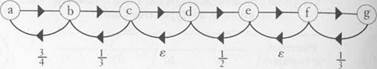 Figure 3.6. A Markov chain with a linear transition structure.
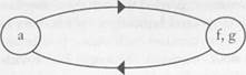 Figure 3.7. Resistances between the two recurrent classes in Markov chain shown in Figure 3.6.
 Figure 3.8. Single disadvantageous trade in segregated state resulting in state with isolated individuals.