CATEGORIES:
BiologyChemistryConstructionCultureEcologyEconomyElectronicsFinanceGeographyHistoryInformaticsLawMathematicsMechanicsMedicineOtherPedagogyPhilosophyPhysicsPolicyPsychologySociologySportTourism
Diffraction and Fresnel ZonesRefraction and reflection of radio waves are mechanisms which are fairly easy to picture, but diffraction is much less intuitive. To understand diffraction, and radio propagation in general, it is very helpful to have some feeling for how radio waves behave in an environment which is not strictly "free space". Consider Fig. 1, in which a wavefront is traveling from left to right, and encountering an obstacle which absorbs or reflects all of the incident radio energy. Assume that the incident wavefront is uniform; i.e., if we measure the field strength along the line A-A', it is the same at all points. Now, what will be the field strength along a line B-B' on the other side of the obstacle? To quantify this, we provide an axis in which zero coincides with the top of the obstacle, and negative and positive numbers denote positions above and below this, respectively (we'll define the parameter used on this axis a bit later).
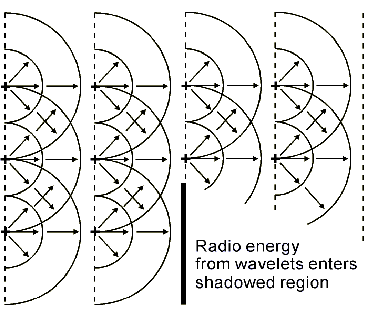
Figure 2 Signal Levels on the Far Side of the Shadowing Object Intuition may lead one to expect the field strength along B-B' to look like the dashed line in Fig. 2, with complete shadowing and zero signal below the top of the obstacle, and no effect at all above it. The solid line shows the reality: not only does energy "leak" into the shadowed area, but the field strength above the top of the obstacle is also disturbed. At a position which is level with the top of the obstacle, the signal power density is down by some 6 dB, despite the fact that this point is in "line of sight" of the source. This effect is less surprising when one considers other familiar instances of wave motion. Picture, for example, tossing a rock in a pond and watching the ripples propagate outward. When they encounter an object such as a boat or a pier, you will see that the water behind the object is also disturbed, and that the waves traveling past, but close to, the object are also affected somewhat. Similarly, consider a distant source of sound waves: if the sound level is well above the ambient level, then moving behind an object which absorbs the incident sound energy completely does not result in the sound disappearing completely - it is still audible at a lower level, due to diffraction (as an aside, it is interesting to note that the wavelength of a 1 KHz sound wave is nearly the same as a 1 GHz radio wave). So much for analogies - let's get back to radio waves. The explanation for the non-intuitive behavior of radio waves in the presence of obstacles which appear in their path is found in something called Huygens' Principle. Huygens showed that propagation occurs as follows: each point on a wave front acts as a source of a secondary wave front known as a wavelet, and a new wave front is then built up from the combination of the contributions from all of the wavelets on the preceding wave front. The secondary wavelets do not radiate equally in all directions - their amplitude in a given direction is proportional to (1 + cos a), where a is the angle between that direction and the direction of propagation of the wave front. The amplitude is therefore maximum in the direction of propagation (i.e., normal to the wave front), and zero in the reverse direction. The representation of a wave front as a collection of wavelets is shown in Fig. 3.
Figure 3 Representation of Radio Waves as Wavelets
Figure 4 Building of a New Wave front by Vector Summation At a given point on the new wavefront (point B), the signal vector (phasor) is determined by vector addition of the contributions from the wavelets on the preceding wave front, as shown in Fig. 4. The largest component is from the nearest wavelet, and we then get symmetrical contributions from the points above and below it. These latter vectors are shorter, due to the angular reduction of amplitude mentioned above, and also the greater distance traveled. The greater distance also introduces more time delay, and hence the rotation of the vectors as shown in the figure. As we include contributions from points farther and farther away, the corresponding vectors continue to rotate and diminish in length, and they trace out a double-sided spiral path, known as the Cornu spiral.
Figure 5 The Cornu Spiral The Cornu spiral, shown in Fig. 5, provides the tool we need to visualize what happens when radio waves encounter an obstacle. In free space, at every point on a new wave front, all contributions from the wavelets on the preceding wave front are present and unattenuated, so the resultant vector corresponds to the complete spiral (i.e., the endpoints of the vector are X and Y). Now, consider again the situation shown in Fig. 1, and for each location on the wave front B-B', visualize the makeup of the Cornu spiral (note that the top of the obstacle is assumed to be sufficiently narrow that no significant reflections can occur from it). At position 0, level with the top of the obstacle, we will have only contributions from the positive half of the preceding wave front at A-A', since all of the others are blocked by the obstacle. Therefore, the received components form only the upper half of the spiral, and the resultant vector is exactly half the length of the free space case, corresponding to a 6 dB reduction in amplitude. As we go lower on the line B-B', we start to get blockage of components from the positive side of the A-A' wave front, removing more and more of the vectors as we go, and leaving only the tight upper spiral. The resulting amplitude diminishes monotonically towards zero as we move down the new wave front, but there is still signal present at all points behind the obstacle, as shown in the graph in Fig. 2. How about the points along line B-B' above the obstacle, where the graph shows those mysterious ripples? Again, look at the Cornu spiral: as we move up the line, we begin to add contributions from the negative side of the A-A' wave front (vectors -1, -2, etc.). Note what happens to the resultant vector - as we make the first turn around the bottom of the spiral, it reaches its maximum length, corresponding to the highest peak in the graph of Fig. 2. As we continue to move up B-B' and add more components, we swing around the spiral and reach the minimum length for the resultant vector (minimum distance from point Y). Further progression up B-B' results in further motion around the spiral, and the amplitude of the resultant oscillates back and forth, with the amplitude of the oscillation steadily decreasing as the resultant converges on the free space value, given by the complete Cornu spiral (vector X-Y). So, in a nutshell, to visualize what happens to radio waves when they encounter an obstacle, we have to develop a picture of the wave front after the obstacle as a function of the wave front just before it (as opposed to simply tracing rays from the distant source). Now we're in a position to talk about Fresnel zones. A Fresnel zone is a simpler concept once you have some understanding of diffraction: it is the volume of space enclosed by an ellipsoid which has the two antennas at the ends of a radio link at its foci. The two-dimensional representation of a Fresnel zone is shown in Fig. 6. The surface of the ellipsoid is defined by the path ACB, which exceeds the length of the direct path AB by some fixed amount. This amount is n
Figure 6 Fresnel Zone for a Radio Link In order to quantify diffraction losses, they are usually expressed in terms of a dimensionless parameter , given by:
where But how do we calculate whether we have the required clearance? The geometry for Fresnel zone calculations is shown in Fig. 7. Keep in mind that this is only a two-dimensional representation, but Fresnel zones are three-dimensional. The same considerations apply when the objects limiting path clearance are to the side or even above the radio path. Since we are considering LOS paths in this section, we are dealing only with the "negative height" case, shown in the lower part of the figure. We will look at the case where h is positive later, when we consider non-LOS paths. For first Fresnel zone clearance, the distance h from the nearest point of the obstacle to the direct path must be at least
where d1 and d2 are the distances from the tip of the obstacle to the two ends of the radio circuit. This formula is an approximation which is not valid very close to the endpoints of the circuit. For convenience, the clearance can be expressed in terms of frequency:
where f is the frequency in GHz, d1 and d2 are in km, and h is in meters. Or:
where f is in GHz, d1 and d2 in statute miles, and h is in feet.
Figure 7 Fresnel Zone Geometry Example 2.We have a 10 km LOS path over which we wish to establish a link in the 915 MHz band. The path profile indicates that the high point on the path is 3 km from one end, and the direct path clears it by about 18 meters (60 ft.) - do we have adequate Fresnel zone clearance? From equation (10a), with d1 = 3 km, d2 = 7 km, and f = 0.915 GHz, we have h = 26.2 m for first Fresnel zone clearance (strictly speaking, h = -26.2 m). A clearance of 18 m is about 70% of this, so it is sufficient to allow negligible diffraction loss. Fresnel zone clearance may not seem all that important - after all, we said previously that for the zero clearance (grazing) case, we have 6 dB of additional path loss. If necessary, this could be overcome with, for example, an additional 3 dB of antenna gain at each end of the circuit. Now it's time to confess that the situation depicted in Figures 1 and 2 is a special case, known as "knife edge" diffraction. Basically, this means that the top of the obstacle is small in terms of wavelengths. This is sometimes a reasonable approximation of an object in the real world, but more often than not, the obstacle will be rounded (such as a hilltop) or have a large flat surface (like the top of a building), or otherwise depart from the knife edge assumption. In such cases, the path loss for the grazing case can be considerably more than 6 dB - in fact, 20 dB would be a better estimate in many cases. So, Fresnel zone clearance can be pretty important on real-world paths. And, again, keep in mind that the Fresnel zone is three-dimensional, so clearance must also be maintained from the sides of buildings, etc. if path loss is to be minimized. Another point to consider is the effect on Fresnel zone clearance of changes in atmospheric refraction, as discussed in the last section. We may have adequate clearance on a longer path under normal conditions (i.e., 4/3 earth radius), but lose the clearance when unusual refraction conditions prevail. On longer paths, therefore, it is common in commercial radio links to do the Fresnel zone analysis on something close to "worst case" rather than typical refraction conditions, but this may be less of a concern in amateur applications. Most of the material in this section was based on Ref. [2], which is highly recommended for further reading. Ground Reflections An LOS path may have adequate Fresnel zone clearance, and yet still have a path loss which differs significantly from free space under normal refraction conditions. If this is the case, the cause is probably multipath propagation resulting from reflections (multipath also poses particular problems for digital transmission systems - we'll look at this a bit later, but here we are only considering path loss). One common source of reflections is the ground. It tends to be more of a factor on paths in rural areas; in urban settings, the ground reflection path will often be blocked by the clutter of buildings, trees, etc. In paths over relatively smooth ground or bodies of water, however, ground reflections can be a major determinant of path loss. For any radio link, it is worthwhile to look at the path profile and see if the ground reflection has the potential to be significant. It should also be kept in mind that the reflection point is not at the midpoint of the path unless the antennas are at the same height and the ground is not sloped in the reflection region - just the remember the old maxim from optics that the angle of incidence equals the angle of reflection. Ground reflections can be good news or bad news, but are more often the latter. In a radio path consisting of a direct path plus a ground-reflected path, the path loss depends on the relative amplitude and phase relationship of the signals propagated by the two paths. In extreme cases, where the ground-reflected path has Fresnel clearance and suffers little loss from the reflection itself (or attenuation from trees, etc.), then its amplitude may approach that of the direct path. Then, depending on the relative phase shift of the two paths, we may have an enhancement of up to 6 dB over the direct path alone, or cancellation resulting in additional path loss of 20 dB or more. If you are acquainted with Mr. Murphy, you know which to expect! The difference in path lengths can be estimated from the path profile, and then translated into wavelengths to give the phase relationship. Then we have to account for the reflection itself, and this is where things get interesting. The amplitude and phase of the reflected wave depend on a number of variables, including conductivity and permittivity of the reflecting surface, frequency, angle of incidence, and polarization. It is difficult to summarize the effects of all of the variables which affect ground reflections, but a typical case is shown in Fig. 8 [2]. This particular figure is for typical ground conditions at 100 MHz, but the same behavior is seen over a wide range of ground constants and frequencies. Notice that there is a large difference in reflection amplitudes between horizontal and vertical polarization (denoted on the curves with "h" and "v", respectively), and that vertical polarization in general gives rise to a much smaller reflected wave. However, the difference is large only for angles of incidence greater than a few degrees (note that, unlike in optics, in radio transmission the angle of incidence is normally measured with respect to a tangent to the reflecting surface rather than a normal to it); in practice, these angles will only occur on very short paths, or paths with extraordinarily high antennas. For typical paths, the angle of incidence tends to be of the order of one degree or less - for example, for a 10 km path over smooth earth with 10 m antenna heights, the angle of incidence of the ground reflection would only be about 0.11 degrees. In such a case, both polarizations will give reflection amplitudes near unity (i.e., no reflection loss). Perhaps more surprisingly, there will also be a phase reversal in both cases. Horizontally-polarized waves always undergo a phase reversal upon reflection, but for vertically-polarized waves, the phase change is a function of the angle of incidence and the ground characteristics.
Figure 8 Typical Ground Reflection Parameters The upshot of all this is that for most paths in which the ground reflection is significant (and no other reflections are present), there will be very little difference in performance between horizontal and vertical polarization. For very short paths, horizontal polarization will generally give rise to a stronger reflection. If it turns out that this causes cancellation rather than enhancement, switching to vertical polarization may provide a solution. In other words, for shorter paths, it is usually worthwhile to try both polarizations to see which works better (of course, other factors such as mounting constraints and rejection of other sources of multipath and interference also enter into the choice of polarization). As stated above, for either polarization, as the path gets longer we approach the case where the ground reflection produces a phase reversal and very little attenuation. At the same time, the direct and reflected paths are becoming more nearly equal. The path loss ripples up and down as we increase the distance, until we reach the point where the path lengths differ by just one-half wavelength. Combined with the 180° phase shift caused by the ground reflection, this brings the direct and reflected signals into phase, resulting in an enhancement over the free space path loss (theoretically 6 dB, but this will seldom be realized in practice). Thereafter, it's all downhill as the distance is further increased, since phase difference between the two paths approaches in the limit the 180° phase shift of the ground reflection. It can be shown that, in this region, the received power follows an inverse fourth-power law as a function of distance instead of the usual square law (i.e., 12 dB more attenuation when you double the distance, instead of 6 dB). The distance at which the path loss starts to increase at the fourth-power rate is reached when the ellipsoid corresponding to the first Fresnel zone just touches the ground. A reasonably good estimate of this distance can be calculated from the equation
where h1 and h2 are the antenna heights above the ground reflection point. For example, for antenna heights of 10 m, at 915 MHz ( So, for longer-range paths, ground reflections are always bad news. Serious problems with ground reflections are most commonly encountered with radio links across bodies of water. Spread spectrum techniques and diversity antenna arrangements usually can't overcome the problems - the solution lies in siting the antennas (e.g., away from the shore of the body of water) such that the reflected path is cut off by natural obstacles, while the direct path is unimpaired. In other cases, it may be possible to adjust the antenna locations so as to move the reflection point to a rough area of land which scatters the signal rather than creating a strong specular reflection. Date: 2016-03-03; view: 823
|


 /2, where n is a positive integer. For the first Fresnel zone, n = 1 and the path length differs by
 (8)
(8) d is the difference in lengths of the straight-line path between the endpoints of the link and the path which just touches the tip of the diffracting object (see Fig. 7, where
  is positive when the direct path is blocked (i.e., the obstacle has positive height), and negative when the direct path has some clearance ("negative height"). When the direct path just grazes the object,
  (9)
(9) (10a)
(10a) (10b)
(10b)

 (11)
(11)