CATEGORIES:
BiologyChemistryConstructionCultureEcologyEconomyElectronicsFinanceGeographyHistoryInformaticsLawMathematicsMechanicsMedicineOtherPedagogyPhilosophyPhysicsPolicyPsychologySociologySportTourism
Numerical simulations of the White Sea hydrodynamics and marine ecosystem
This chapter presents recent advances in numerical modeling of the hydrodynamics and marine ecosystem of the White Sea. Section 10.1 puts forth a hydrodynamic numerical modeling effort performed at the Nansen Environmental and Remote Sensing Center (NERSC), Bergen, Norway. Section 10.2 describes a 1-D ecological model by the Finnish Institute for Marine Research (FIMR), Helsinki. Another model from FIMR - a more complex, mixotrophic ecosytem model - is presented in Section 10.3. Section 10.4 describes a different sort of model developed by the Institute of Oceanology (IO), Russian Academy of Sciences (RAS). Section 10.5puts forth a hydrodynamic model developed jointly by the St. Petersburg branch of IO/ RAS and the Arctic and Antarctic Research Institute (AARI), St. Petersburg, Russia. Section 10.6 discusses the response of the White Sea ecosystem to future climate change and its feedback on socio-economic conditions. Finally, a number of conclusions are made in Section 10.7.
10.1 NERSC-HYCOM HYDRODYNAMIC MODEL
10.1.1 Model overview
The NERSC model simulations have used a version of the Hybrid Coordinate Ocean Model (HYCOM), developed at the University of Miami, Florida, USA. HYCOM is an ocean general circulation model (GCM) that can combine various types of vertical coordinates, viz. density-governed isopycnic ( p), bottom-governed sigma (o), and level (z) coordinates (Bleck, 2002). Theoretically, this should provide the possibility for a sound simulation of a wide spectrum of oceanic conditions: from a stratified ocean to boundary mixed regions.
Isopycnic surfaces were set to be the main vertical coordinate system in the model, since they simulate the well-known property of water in a stratified ocean
to move following the isopycnals (i.e., surfaces of constant density) with compara- tively weak diapycnal mixing.
Bottom-following o-coordinates were included for the regions where the bottom topography plays a leading role in ocean dynamics, such as the density overflow systems (Evensen, 1997). The surface/bottom mixed layer (as deep as the convection region in the Greenland Sea, and as large as tidally mixed coastal shoals) can be represented in z-coordinates (Bleck, 2002). Though comparatively negligible compared with the ocean water volume, those areas are extremely important for the ocean water mass formation, as well as for marine life. A smooth transition between various coordinate systems is ensured in the model via the so-called
cushion functions , which are dependent on layer thickness (Langlois, 1997). At the same time, stipulating predominantly anisopycnic ocean behavior, one should be very careful with the vertical discretization of the model domain. For example, in order to model narrow flows trapped in the vicinity of a deep bottom, taking into account weak water stratification below the main thermocline, very accurate near- bottom vertical density layering should be done. Enhanced horizontal cross- frontal mixing (as compared to the interior diapycnal mixing) as well as mesoscale cross-isopycnic mass and energy transport (by internal tides and inertial waves (Konaev and Sabinin, 1992)) are taken into consideration in the HYCOM by making diffusion coefficients dependent on horizontal and vertical shears and, thus, becoming enhanced in the regions of strong shear currents. The threshold value from which the shear mixing starts exerting its effect has to be watched.
The HYCOM equations with a generalized vertical coordinate (s) are written below in the same order, as being numerically solved in the model (e.g., the mass conservation, thermodynamic variables conservation, and horizontal momentum equations) (Bleck et al., 2002):
8

8ts
( 8p \

8s
+ V's ·
( 8p\

|
8s
8 ( 8p \

 s
s
8s 8s
= 0 (10.1)
8 ( 8 p R\
( 8 p \
R +
8(s
8p R\
(
= V's ·
8p
\
V'sR
+ HR (10.2)
8
8ts
8s
+ V's ·
8s 8s 8s 8s
8p \ 8
+ f )k x + (
+ M - p o: =

 8ts+ V's 2 +(
s

 8p 8p
8p 8p
V's
8 T
 -g 8p+
V's
( 8p\-1
8s
V's ·
( 8p \
|
(10.3)
Those are complimented by diapycnal mixing and layer interface vertical dis- placement equations:
( 8 \
( 8p 8 p \ 8
8(K
8\
10.4
|
8t 8p
8p = - 8p 8z ( )
|
8(8p8p \ 0
10.5
8t 8p
+ 8p
8t 8p = ( )
The system is closed with the hydrostatic equation and a simplified equation of state:
8M
 8o: = p (10.6)
p(T , S, p) = C1(p)+ C2(p)T + C3(p)S + C4(p)T 2
+ C5(p)ST + C6(p)T 3 + C7(p)ST 2 (10.7)
where s is either the p-, z-, or o- coordinate; p = water density; p = pressure; V(u, ) = is the northward or eastward velocity; R is a thermodynamic variable (e.g., water temperature (T ) or salinity (S)); = horizontal diffusivity; Ht = sum of diabatic flux terms, including diapycnal mixing; = 8 /8x - 8u/8y = relative vorticity; f "' sin(<p) = Coriolis parameter; <p = latitude; k = vertical unit vector; M = gz + po: is the Montgomery potential g = gravity acceleration; o: = 1/p;
( 8p 8p \
T = surface/bottom drag;

8t 8p
= generalized vertical velocity; Ci= pressure
|
This system of non-linear hydrodynamic equations for a hydrostatic Boussinesq fluid can describe most of the large and medium range ocean phenomena occurring, including wind and density driven circulation, frontal dynamics, ocean eddies and waves - up to short-period wave motions, where a hydrostatic approximation does not hold. Tidal phenomena can be added to the system, provided a space-time depending horizontal component of the force generating the tide in the right-hand side of the momentum equation is available.
A numerical solution implies space-time discretization of the equations. Hori- zontal discretization limits the number of phenomena that can be described to the ones at horizontal scales several times bigger than the size of the model horizontal mesh cell (!ix).
 Thus, to resolve mesoscale wave/vortex phenomena, the Rot» !ix criterion (where Rot= ct/f is the internal Rossby-Obukov radius, ct= jgtH is the phase
speed of long internal gravity waves, gtis the reduced gravity, and H is the water depth) is to be satisfied (Kantha and Clayson, 2000a). The model equations are solved on the Araquava C-grid, where thermodynamic variables as well as the northern and eastern current velocity components are scattered in space to reduce the effect of spatial discontinuity in model equations. The use of the C-grid reduces the dispersion of the desired numerical solution, provided the internal Rossby- Obukov radius (Rot) is in excess of the model horizontal mesh resolution (Adcroft et al., 1999). Together with the method of ghost points for non-slip boundary conditions, implemented in the HYCOM, the C-grid can cause the hori- zontal viscous stress to be underestimated at solid boundaries. To reproduce ade- quately the frontal dynamics, it is also important that in the continuity equation the
frontal zones be well resolved: b = l!ix/p bp/bxl« 1, where bp/bx is the mean horizontal density gradient in the frontal zone (Kantha and Clayson, 2000a).
In the vertical, a suitable choice of model density layers assures high vertical resolution inside the isopycnic domain. In the z domain, setting up of the minimum z-layer thickness parameter (bz) assures the mixed layer always to be present during the mixed layer detrainment process. A judicious choice of a maximum z-layer thickness parameter (bzm) gives the possibility of obtaining a better resolution for a thick (> bzm) mixed layer by incorporating near-surface, zero-thickness isopycnic layers in the z-coordinate mixed layer domain. In the o domain, one is able to specify the sea depth interval (Homin, Ho max), within which the ocean
- -
dynamics will be represented in o- coordinates using the following expressions:
Ho min = bo No, and Ho max = bz No, where bo is the minimum o-layer
- -
thickness and Nois a maximum total number of o-layers.
The prognostic variables are interpolated to the new grid in a manner conserving the corresponding vertical integrals. A vertical resolution, if insufficiently low, can limit an adequate representation of narrow flows and the vertical wave mode for internal waves. Special attention needs to be paid to the isopycnic domain, where the boundaries of layers are migrating on a seasonal basis.
Time discretization implies an algorithm to be numerically stable if only the model Courant number (Cu = !it/!ix) is small enough. As for the flux- corrected transport (FCT) algorithm (Boris and Brook, 1973; Zalesak, 1979), used for the solution of the continuity equation, the algorithm is stable if Cu ::; 0.5. The MPDATA algorithm, used for the solution of T S/advection equations, is stable if the sum of Courant numbers in all coordinate directions is under 0.5 (Drange and Bleck, 1997).
The bottom boundary layer thickness in the model is predetermined (typically 10 m) and sets up a limit to the minimum water depth, which could be specified for computations. However, in the case of vast shallow areas, this can force the simulated coastline to differ from the real one.
|
|
V'!ipt), and
|
!iptV' ), of a k-layer are incorporated in the flux term,
|
|
the model horizontal turbulent diffusion coefficient on the horizontal spatial scale
u = Udu !ix is not very different from the 4/3 law, observed in the ocean:
u "' E1/3 !ix4/3(Ozmidov, 1986), where the turbulent dissipation rate (E) is taken to be constant (Kantha and Clayson, 2000b).
After the horizontal advection is simulated and new velocity fields are computed, the vertical diapycnal mixing is included. The task is now reduced to a 1-D vertical mixing equation at the layer interfaces. Three vertical mixing schemes are available. The main K-Profile Parameterization (KPP) scheme did not conserve the layer reference density and later required re-gridding. Based on the K-theory, the coeffi- cient of vertical diffusivity is constituted by 3 components, viz. the term of local velocity shear, mixing term inherent in subgrid internal waves, and double diffusion term. The equations of vertical diffusion are solved simultaneously for all isopycnic layers in an iterative way to take into account the local buoyancy being reduced in the course of vertical mixing.
Due to incorporation of non-local diapycnal mixing, this method overcomes the general drawback of isopycnic models, which often arises from underestimation of diapycnal mixing in the regions of strong entrainment (Griffies et al., 2000). This scheme also works reasonably well for a rather coarse vertical model resolution (Large et al., 1994). At the same time, utilization of local instantaneous profiles of p and V renders the KPP approach not very stable, especially in the initial stage of computations when it is better replaced with the explicit algorithm , included in the HYCOM. Due to the processes of diapycnal mixing and cabbeling, the layer density at a grid point changes, conflicting with the demand for the layer reference density to be maintained to the end of the integration. A procedure of vertical re-gridding is applied to restore the layer density after each time step: if the density of a layer becomes out of range, one of the layer interfaces is moved either to dilute it with lighter water from the above or with denser water from below. In the case of an excessively light bottom layer, it is divided into the upper sub-layer with density equal to that of the adjacent upper layer, and the lower of the desired reference density. Re-gridding induces artificial numerical mixing, especially in the upper ocean with high variability in layer thickness (Bleck, 2002).
The dynamics of the surface mixed layer does not have a reference density, since its properties are constantly modified by external forcing. The surface forcing is bound to surface heat, freshwater, and momentum fluxes. Snow and sea ice cover effect is included, which modifies surface forcing, if the surface water temperature falls below freezing point and the resulting ice thickness hice averaged over the grid cell exceeds a certain minimum. The dynamics of old ice is governed by both the heat/water balance at the upper and lower surfaces of sea ice and the thermodynamic fluxes through the ice.
Ice hummocking is included in a manner that conserves the overall ice volume. River discharge directly affects the sea level and salinity of the water surface layer at the 3-point areas adjacent to the river mouth. The depth of the mixed layer is governed by two main external factors, viz. surface buoyancy flux (B) and wind stress (T ). The surface wind stress governs the depth of the mixed layer until it exceeds the depth of the Ekman layer, when, in turn, a convective instability starts
to take the leading role. Bottom and wind stresses in the model are taken in a standard quadratic form. The KPP (based on Monin-Obukov theory) or modified Krauss-Tuner (KT) algorithms (Krauss and Tuner, 1967) are available. The mixed layer depth in hybrid coordinates does not generally correspond to a layer interface depth and constant re-gridding of the upper layers (mixed layer with the glued mass- less layers of low-reference densities and the first isopycnic sub-layer) leads to diffus- sion effects (Bleck, 2001).
Barotropic inertial-gravity waves (e.g., tidal waves) are simulated through gen- erating barotropic currents arising from sea level gradients in the barotropic equations, which, in turn, would result in the propagation of sea level fluctuations inside the model domain through current divergence. In the case of a flat bottom, the above terms completely balance each other and do not produce any internal disturb- ances. If for some reason a flow goes across the isobaths, either down or up the slope, and it is not immediately balanced by the horizontal current divergence, the sea level will fall/rise locally. This change of the sea level will affect the internal layers, for which a relative change of layer thickness is proportional to the sea level change. Thus, a barotropic wave will loose a certain part of its energy through powering internal oscillations, which is consistent with the theory of generation of the internal tide.
Non-linear equations of water motion allow overtone wave generation (shallow- water waves in the tidal terminology), through current-sea level, current-current, and friction non-linearity. For the purpose of the correct treatment of horizontal pressure force (V'M), if a layer intersects the bottom relief profile, the later is considered to be constant in a mesh cell. This limits the forms of shelf waves, which would appear in the model as Kelvin or flat-shelf modes. The sloping- shelf modes would appear only if the shelf width is greater than the mesh size by an order of magnitude.
In the isopycnic model of UNESCO-83, a simple analytic parameterization of the equation of state is a necessity for a fast numerical scheme. The polynomial approximation in the HYCOM holds well for a wide range of water temperature and salinity. At the same time, it gives an understated temperature for the maximum density of seawater, which in the HYCOM equation of state is 0.6oC lower than in reality. This is highly consequential at water salinity values under 24.690, when the temperature of maximum density exceeds the seawater freezing point and the freezing waters are no longer the densest. In the HYCOM approximation of the equation of state this critical salinity value is not 24.690, but lies close to
210. Thus, in the HYCOM, at salinities of about 21-240, the seawater reaches its maximum density at too low a (freezing) temperature (Figure 10.1). In polar coastal areas, where the water salinity can be below 240, this discrepancy would produce stronger vertical mixing during the entire period of sea surface freezing.
10.1.2 The HYCOM implementation for the White Sea
These analyses have shown that the HYCOM can adequately describe water density variations as well as the flow dynamics controlled topographically, which is the case
|
 Figure 10.1. Correspondence between the water freezing temperature (Tfr) and the temperature of maximum density (Tmd) for the UNESCO-83 and HYCOM equations of state.
for the general circulation in the White Sea. It can also adequately describe the inherent non-linear tidal dynamics, which is an important source of horizontal and vertical mixing in the sea.
In winter, the salinity of surface water is high enough (> 270) to exclude the effect of excessive vertical mixing, which can occur only in some limited coastal regions and will not play a decisive role in sea dynamics. So with an appropriate model configuration it is possible to expect a reasonable simulation of seasonal dynamics in the White Sea.
The White Sea HYCOM was set up for the most detailed topography of the region available (NIERSC-TRANSAS data set, see Chapter 1). For the reduction of undesirable effects while implementing the o-coordinates, the marine topography was smoothed by the second-order Savitzky-Golay filter. During gridding, one- point islands and inlets were eliminated to avoid the related instabilities and spurious drag. For attaining the stability of the numerical solution, a minimum depth was set to be 20 m. This, in turn, resulted in flattening of the topography in the shallow Mezenskiy and Onezhskiy Bays requiring some tuning of the coastline to restore the configuration of the coastlines of the above bays and conserve the overall water volume. Table 10.1 indicates that the mean characteristics of the White Sea Basin have not significantly changed following on from the above simplifications.
From the normalized histograms of the distribution of White Sea depth (Figure 10.2), it can be concluded that, apart from a slight shift from average to
Table 10.1. Topographic characteristics of the White Sea Basin as reported in the literature (Hydrometeorology ... , 1991) and as used in the model.
| Characteristic | In the literature | In the model |
| Surface area (km2) Average depth (m) | 0.09 x 10659 | 0.09 x 10656 |
| Maximum depth (m) |
An abrupt one-point fall in Kandalakshskiy Bay was smoothed by the filter.

Figure 10.2. Normalized histograms for water depth ranges (in meters) in the NIERSC- TRANSAS data set and the smoothed data used in the White Sea HYCOM. The difference between histograms is plotted on the right-hand side.
small depths, the applied simplifications have not substantially changed the general depth frequency distribution.
The model mesh was rotated with respect to the geographical coordinates (Bentsen et al., 1999), so that the model poles were placed outside the model domain to avoid pole-related singularities. Additionally, the horizontal mesh was set up in order to align much of the coastline with the mesh lines. This was designed to reduce possible spurious drag at the ghost points at the solid boundaries of the
|
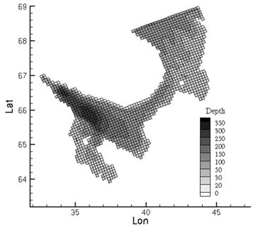
Figure 10.3. Contours of the model mesh and depth (m). Only every second meshline is shown.
Arakawa C-grid. Special attention was paid to the Gorlo coasts, where the exchange of the White Sea water with the Barents Sea is of basic importance for the dynamics of the White Sea (Figure 10.3).
The mesh resolution was approximately 4 km x 4 km across the domain. This permits resolution of the inertia-gravity waves on the C-grid for sea depths exceeding 50 m, where the baroclinic Rossby radius of deformation is about 10-30 km.
At the same time, a lower horizontal resolution is desirable for vast shallow areas. Frontal zones are also one of the important issues of the dynamics of the White Sea since they limit the horizontal water exchange with the bays and the Barents Sea. A stability criteria for divergent flows in the zones of sharp density gradients b = l!ix/p dp/dxl « 1 was not satisfied for frontal zones in the White Sea (b is 4 for the Dvinskiy Bay front and 1 for the other fronts). This means smearing of the fronts, though the applied weakly diffusive FCT (Boris and Book, 1973; Zalesak, 1979) and MPDATA (Drange and Bleck, 1997) numerical schemes add to the conservation of high gradients in the frontal regions. The time step used in the theoretical model based on the Courant number has to be less than 10 min. Our simulation has showed that during winter the model is stable if the step is only about 2 min.
An adequate simulation of the water exchange with the Barents Sea, primarily controlled by the sea level variations, is of great importance for the dynamics of the
White Sea (Altshuler and Sustavov, 1970). To obtain the boundary conditions, the domain of the White Sea was nested into the DIADEM, which is a HYCOM-type model, implemented at NERSC for simulating the Atlantic and the Arctic Oceans (Evensen and Johannessen, 2000). A comparison of the DIADEM with data from observations (Furevik, 2001) showed a good agreement between mean monthly and seasonal variability, though the water temperature in the model is a bit higher than the observed. At the White Sea boundary, the DIADEM had an approximately 26 km x 26 km horizontal mesh resolution, which is nearly that required for an appropriate nesting of a 4-km model. The results of simulations showed that spurious oscillations near the boundary are reasonably small and the mean circula- tion in the area is close to that derived from in situ observations. The relaxation boundary conditions, pressure nudging, damping of the pressure term in the con- tinuity equation, and enhanced viscosity were applied in the 20-point relaxation domain. At the boundary, the nested model was forced by the DIADEM baroclinic and barotropic pressure, velocity, as well as temperature and salinity. Ice exchange at the boundary was disregarded. The Atlantic heat transport to the Barents Sea makes the model boundary practically ice-free during the entire year and the negative net heat exchange owing to sea ice advection comprises only 3% of the heat balance inherent in the total sea surface (Arsenieva, 1964).
Barotropic and baroclinic velocities at the open boundary are treated separately. The barotropic normal to the boundary velocity vector are obtained from the Browning-Kreiss boundary conditions, where barotropic waves are radiated through the boundary using the method of characteristics. Tangential barotropic velocities and baroclinic velocities at the boundary are prescribed to satisfy the hydrodynamic equations. This permits a proper treatment of the incoming/ reflected barotropic inertia-gravity waves at the boundary without generation of a strong spurious computational mode. The algorithm used for the dynamic boundary condition permits addition of the tidal oscillations to the low-scale sea level varia- tions taken from the DIADEM.
In the White Sea, the tidal motions are an important source of vertical mixing. According to available observations, the resultant tidal oscillations at the entrance of the Voronka are about 2-3 m high and the tide loses more then 70% of its energy in the Voronka and Mezenskiy Bay. The rest of the arriving energy is mainly dissipated in the Gorlo and Onezhskiy Bay (Altshuler and Sustavov, 1970). The tidal wave non- linearity results in residual tidal currents, which, in some marine areas, can have the same velocities as the velocities of the mean seasonal circulation (Hydrometeorology
.. ., 1991). The tides in the White Sea can be adequately modeled by forcing at the boundary only. Sea level oscillations for 8 main tidal waves (K1, O1, P1, Q1, M2, S2, N2 and K2) were imposed on the northern Voronka. Harmonic constants at the boundary were taken from the results of the FES model (Lefevre et al., 2000), which is in good agreement with the tidal maps based on in situ observations (Hydro- meteorology .. ., 1991). Tides in shallow waters play an appreciably important role in some inner parts of the White Sea. However at the boundary, they are less than 1% of M2 amplitudes and thus can be ignored (Hydrometeorology .. ., 1991). Our simulations for the inner regions result in a generation of shallow-water tides. This is
|
due to non-linear terms in the momentum equations. According to the available observations, the above tides absorb up to 25% of the M2 tidal energy in the vast shallow regions of the White Sea.
In the isopycnic domain, vertical layering in the model was chosen to coincide as close as possible with that of the outer DIADEM. Special attention has been paid to cover the typical density ranges of water masses in the White Sea below a 10-m mixed layer (21-26 kg m-3in the open sea and up to 28 kg m-3in the Voronka), preferably having some isopycnic layer boundaries coinciding with those of the existing water masses. 22 isopycnic layers were used. These layers were assumed to have the following densities (in kg m-3): 19.00, 20.50, 21.60, 22.20, 23.05, 23.55,
24.05, 24.20, 24.50, 24.75, 24.96, 25.10, 25.30, 25.68, 26.25, 26.69, 27.03, 27.29,
27.49, 27.66, 28.02, and 28.11. Given the DIADEM configuration, the minimum vertical thickness of z-layers (bz) was taken to be 10 m. The maximum vertical thickness of z-layers (bzm) was also set up at 10 m, to get a better resolution of the upper mixed layer in winter.
The o-coordinates were used to cover the depth range of 24-60 m (6 o-levels with a minimum layer thickness of 4 m). This assures a better treatment of topographic- ally governed density inflow in the tidally mixed regions of the Gorlo and Voronka, while most parts of the flat and vertically homogeneous tracts of Onezhskiy and Mezenskiy Bays are treated in the z-coordinates.
In order to take the external atmospheric forcing into account, data from ECMWF reanalysis of a 6-hour air temperature, the temperature of dew point (as a measure of precipitation), and wind velocity were used (ECMWF, 2002). Cloudi- ness data were taken from the available climatic data for the region. Special attention was paid to a proper treatment of river inflow, which creates most of the specific features of hydrodynamics in the White Sea. Nine main rivers were included in the model, namely: Severnaya Dvina (49.6%), Mezen (10.8%), Onega (7.9%), Kem (together with Nizhny Vyg) (7.6%), Kovda (together with Umba and Neva) (4%), and Ponoy (2.8%) (Annual .. ., 2001). The above rivers account for a total discharge of "' 185km3 yr-1(i.e., 82% of the overall river discharge, which is about 225km3 yr-1. To comply with the total freshwater inflow observed, the remaining 18% of small river discharges were proportionally distributed among the main rivers, in accordance with the values of river discharges assessed for the total coastal area (Elshin, 1979). The seasonal variability of discharge was set up individ- ually for each of the rivers (Annual .. ., 2001). Most of the rivers exhibit a strong discharge peak in May-June.
Since the water salinity plays a major role in the formation of the White Sea stratification and water dynamics, the S and p variables were used for calculation of the vertical grid in the isopycnic domain, but the T and S variables were advected. For this configuration, the vertical re-gridding process does not always result in full conservation of heat in the marine water column, but suppresses cabbeling (Bleck, 2002), which should somewhat compensate for non-physical numerical mixing. The conducted numerical experiments showed that the model is immune to emerging changes in the leading thermodynamic variables due to the re- gridding procedure.
10.1.3 Model experiments
Utilization of the HYCOM as a high-resolution model for a semi-closed tidal sea demands a careful reconsideration of the model parameters used. The parameters to change were the coefficients used for semi-empirical parameterizations of turbulent mixing fluxes in the HYCOM. For the White Sea coastal simulations, the coefficients can differ from those determined in an open ocean model due to both unequal resolution in the horizontal and vertical directions, and intensive tidal dynamics. Horizontal mixing is especially important in the Gorlo passage, where it can limit the intensity of water exchange with the Barents Sea. The latter determines the vertical stratification in the White Sea. The horizontal diffusion coefficient ( d ) in the model is dependent either on diffusion velocity Ud (e.g., the subgrid background shear, which is spatially uniform), or on the dimensional multiple (,\) in the hori- zontal shear dependent viscosity term:
 ( I( du
d \2
( d
du \2
|
- dy
+ dx + dy
(10.8)

 Keeping Ud» ,\ results in a pronounced horizontal shear instability, but has nearly no effect on the horizontal turbulence, which is not correct from the hydro- dynamic point of view. Naturally, if we set the two terms in d to be equal, then Ud = ,\ !ix (bU/bx), where !ix is the measure of the model horizontal resolution and bU/bx is the local horizontal velocity gradient. Based on the results reported by Kantha and Clayson (2000b), one can conclude that ,\ equal to 1 is a universal constant independent of the model resolution. For the model resolution of 100 km, setting Ud at 2 cm s-1will only result in small gradients in the horizontal velocity (e.g., not having an effect on the horizontal turbulent exchange), if bU/bx ::; Ud /(,\ !ix) "' 10-6s-1, which is an order of magnitude less than the hori- zontal velocity gradient in the ocean frontal zones (10-4-10-5s-1). If we leave Udunchanged and increase the horizontal resolution up to 4 km, the horizontal velocity gradients become negligible at bU/bx ::; 10-4s-1, with the result that d remains the same over the entire model domain. It is easy to see that the diffusion velocity can be written as Ud = d /!ix "' E1/3!ix1/3, where d "' E1/3A4/3, E is the energy of momentum dissipation and A = !ix is the typical length scale for the sub-grid diffusion. In our case of substantial mesh refinement in the nested model, the value of Udshould change proportionally to {(Eo!ixo)/(Ews!ixws)}1/3(here !ixocorresponds to a 100-km ocean model and !ixws to the White Sea 4-km model) or else Ud ws "' 3(Eo/Ews)1/3} Ud o. For the White Sea, with the enhanced tidal dis-
- -
sipation, one could expect that Eo < Ews and the coefficient of proportionality should
be <3. The simulated horizontal hydrodynamics also can be tuned by changing the diapycnal mixing parameters, with the result of modifying the friction between the vertical model layers.
The White Sea horizontal circulation was reconstructed on the bases of in situ observations conducted mainly during the warm season. Thus, a comparison with model results addresses mainly summer months. The surface circulation in the White
|

Figure 10.4. (left) The surface circulation in the White Sea based on in situ data. (right) The circulation in the White Sea at a depth of 100 m.
(left) From Annual (2001); (right) from Lednev (1938).
Sea is mainly cyclonic (Hydrometeorology .. ., 1991) with the feeding current following the Terskiy coast (the north-western coast of the Gorlo) and then heading to the northern coast of Kandalakshskiy Bay. There the flow turns south- eastward and passes by the Karelskiy coast, reaches Onezhskiy Bay, and further runs along Dvinskiy Bay and the Zimniy coast. In the Voronka, the main surface current enters the central part, then turns to the east to finally exit the model area near the Kanin Nos cape (Figure 10.4). In most of the bays, a cyclonic circulation dominates. In the central part of the Bassein, a big anticyclonic vortex is formed, called a center of warmth , but it stands out in the circulation pattern revealed at 100 m depth (Lednev, 1938).
Our tuning experiments have indicated that neither advection nor hybrid generator flags seriously affect the White Sea dynamics, but the model behavior significantly depends on the mixing parameters. The initial set-up of mixing param- eters for the White Sea model is presented in Table 10.2 and those used in some of the tuning experiments are presented in Table 10.3. The model initial run lasted 10 years to reach a stable water circulation and water mass distribution. Starting from this initial state, our numerical experiments were conducted, each lasting about 34 years to stabilize the system in each special case.


 Table 10.2. Initial layering and mixing parameters for the White Sea HYCOM.
| Type of parameter | Parameter | Value |
| nhybrd = number of hybrid levels | ||
| nsigma = number of sigma levels | ||
| dp00s = sigma spacing minimum thickness (m) | 4.0 | |
| dp00 = z-level spacing minimum thickness (m) | 10.0 | |
| dp00x = z-level spacing maximum thickness (m) | 10.0 | |
| viscos = deformation dependent viscosity factor (,\) | 0.1 | |
| veldff = diffusion velocity (m/s) for momentum dissipation (Ud) | 0.005 | |
| thkdff = diffusion velocity (m/s) for thickness diffusion (Ud) | 0.005 | |
| temdff = diffusion velocity (m/s) for temperature/salinity mixing (Ud) | 0.005 | |
| shinst = activate shear instability mixing | true | |
| dbdiff = activate double diffusion mixing | true | |
| nonloc = activate non-local mixing at the mixed layer base | true | |
| rinfty = critical Richardson number (shear instability mixing) | 0.4 | |
| difm0 = maximum viscosity due to shear instability (m 2/s) | 01.e-4 | |
| difs0 = maximum diffusivity due to shear instability (m 2/s) | 01.e-5 | |
| difmiw = background (internal waves) viscosity (m 2/s) | 0.e-4 | |
| difsiw = background (internal waves) diffusivity (m 2/s) | 0.e-5 | |
| dsfmax = salt fingering diffusivity factor (m 2/s) | 0.e-4 | |
| rrho0 = double diffusion density ratio (Rp) | 1.9 | |
| ricr = critical bulk Richardson number at the mixed layer base | 0.2 |
 The results of the first 5 experiments are presented in Figures 10.5 and 10.6. As seen, given the initial parameters (WH1 experiment), the structure of the sea currents are sufficiently well reproduced in the Voronka and Gorlo as well as in Mezenskiy Bay. At the boundary of the model area, the currents are slightly messy , probably due to the inconsistency in model resolution between the outer and inner (nested) models. However, the main pattern of the White Sea water outflow in the Barents Sea is well reproduced. The general cyclonic circulation in the White Sea is, perhaps, overly pronounced because the anticyclonic vortex in the centre of the sea becomes unduly suppressed. The waters of the bays are also involved in a cyclonic movement. The velocities of surface non-periodic currents (10-20 cm s-1) are also consistent with the available observations. The tuning experiments showed that a reduction of the horizontal mixing (Figure 10.5) has brought some intensification of the cyclonic circulation in the Bassein.
This is consistent with results of the Munk theory of a simplified general circula- tion (driven by water density, bottom topography, and the {3-effect (Kantha and Clayson, 2000a)). In the bottom it is seen that a further decrease of horizontal mixing strongly accelerates the eddy to a degree that it becomes unstable and splits into several others. An increase in the horizontal viscosity coefficients
|
Table 10.3. Mixing parameters used in the model tuning experiments (see Table 10.2 for the employed abbreviations).
| Designation of | viscos | veldff (Ud) thkdff | shinst ( difm0 , difs0 ), dbdiff | rinfty ricr | |
| the experiment | (,\) | temdff | nonloc | difmiw , difsiw | nsigma |
| WH1 (initial) | 0.10 | 0.005 | T (1 10-4, 1 10-5) | 0.4 | |
| 0.005 | T | 0.2 | |||
| 0.005 | T | 1 10-4, 1 10-5 | |||
| WH4 | 0.05 0.001 | T (1 10-4, 1 10-5) | 0.4 | ||
| 0.001 | T | 0.2 | |||
| 0.001 | T | 1 10-4, 1 10-5 | |||
| WH5 0.01 | 0.0001 | T (1 10-4, 1 10-5) | 0.4 | ||
| 0.0001 | T | 0.2 | |||
| 0.0001 | T | 1 10-4, 1 10-5 | |||
| WH7 | 0.2 | 0.005 | T (1 10-4, 1 10-5) | 0.4 | |
| 0.005 | T | 0.2 | |||
| 0.005 | T | 1 10-4, 1 10-5 | |||
| WH8 | 0.2 | 0.01 | T (1 10-4, 1 10-5) | 0.4 | |
| 0.01 | T | 0.2 | |||
| 0.01 | T | 1 10-4, 1 10-5 | |||
| WHc | 0.10 | 0.005 | T (1 10-4, 1 10-5) | 0.2 | |
| 0.005 | F | 0.2 | |||
| 0.005 | F | 1 10-6, 1 10-7 | |||
| WH9 | 0.10 | 0.02 | F | 0.2 | |
| 0.02 | F | 0.2 | |||
| 0.02 | F | 5 10-6, 5 10-7 | |||
| WHf | 0.10 | 0.02 | F | 0.2 | |
| 0.02 | F | 0.2 | |||
| 0.02 | F | 1 10-5, 1 10-6 |
Some of the experiments were put in italic and/or bold to unite them in one group.
(Figure 10.6) weakens the general circulation without substantially changing its structure. In both sets of experiments the vertical stratification does not show any significant changes.
The increase in horizontal viscosity coefficients lead to a slight decrease of the surface salinity in the central part of the Bassein due to the suppression of the upwelling inherent in the weakened cyclonic circulation.
The experiments failed to reproduce the central anticyclonic eddy in the Bassein observed in situ, which proved to be replaced by a cyclonic circulation typical of
 | |
 |
|
|
| |
 Figure 10.5. Model experiments: WH1 (top), WH4 (middle), WH5 (bottom). Horizontal mixing decreases from top to bottom. Counts (with 20 intervals) represent the sea surface salinity ranging from 220 at the western part of Dvinskiy Bay to 280 in the Bassein.
|
 | |||
| |

 Figure 10.6. Model experiments: (top) WH1, (middle) WH7, (bottom) WH8. Horizontal mixing increases from top to bottom. Counts (with 10 intervals) represent sea surface salinity from 220 at the western part of Dvinskiy Bay to 280 in the Bassein.
deeper levels in the White Sea. This warrants a conjecture that our model suffers from excessive vertical mixing. This is bound to lead to strong interactions between the upper and lower layers in the sea.
Vertical mixing, water masses and frontal zones
The vertical structure of the White Sea is illustrated in Table 10.4. Except for the river mouths, the Atlantic (AtlWM) and Arctic (ArWM) water masses are dominat- ing. The former is formed due to vertical mixing of fresh river water with the Barents Sea water and occupy the upper layer during the event of maximum convection in winter, typically reaching 35-50 m. The ArWM is formed by the inflow of the Barents Sea water, being modified in the vertically mixed area in the Gorlo. The upper 10-m layer in the AtlWM represents the upper mixed layer in summer with the most significant variability in water temperature and salinity. At a depth of 10-25m a strong pycnocline is formed in summer, abating vertical mixing, which results in a reduced seasonal variability. The seasonal variability of the ArWM is comparatively small and depends on the seasonal changes of water properties in the Barents Sea. The comparison of the modeled (WH1) and the observed stratification showed that the model gives excessive mixing in the vertical, which results in higher salinities in surface waters (>280 instead of 27-280) and lower salinities in the bottom layer (290 instead of 300). Our WHc, WH9, and WHf experiments were intended to study the influence of vertical mixing intensity parameters (Table 10.3). To reduce
Table 10.4. Water masses inherent in the White Sea.
From Hydrometeorology ... (1991).

| WINTER SUMMER | |||||||
| Name of the water mass | o (g cm-3 ) | o (g cm-3) | |||||
| or the layer | dH (m) | T (o C) | S (0) | 10-3 + 1 | T (o C) | S (0) | 10-3 + 1 |
| Atlantic water mass (AtlWM), 0 35 m (up to 70 m ) | |||||||
| AtlWM upper layer | 0-10 | -1 | 20.93 | 17-26 | 11.82 | ||
| AtlWM middle layer | 10-20 | 21.76 | 20.04 |
AtlWM lower layer 20-35 -0.8 27 21.82 5 27 21.48
Arctic water mass (ArWM), below 35 m
ArWM upper layer 35-75 -1.5 28 22.74 2.5 27 21.79
| ArWM middle layer | 75-200 | -1. | 29.5 | 24.20 | -1 28.5 23.38 | ||
| ArWM lower layer >200 -1.5 30 25.18 -1.5 30 25.18 | |||||||
| Estuary water masses, 0 5 m | |||||||
| Estuary - Arctic water mass | 0-5 | -1 | 12.87 | 3-16 | 2.24 | ||
| Estuary - Atlantic water mass | 0-3 | -1 | 12.87 | 3-16 | 0.58 |
In the Gorlo and Onezhskiy Bay.
Notes: dH = depth interval; T, S, and o are the characteristic temperature, salinity, and density, respectively.
|
 Figure 10.7. The vertical profile of water salinity (0) along the Bassein (north of Dvinskiy Bay)-Kandalakshskiy Bay transect. (upper) Observed typical salinity profile in summer. (lower) WH9 model experiment salinity for the summer of 1989. The horizontal line stands for a characteristic position of the conditional demarcation between the Atlantic and Arctic water masses.
vertical mixing, the diapycnal diffusivity was assumed to be controlled exclusively by mixing of spatially uniform internal waves of low intensity. The critical Richardson number was reduced and the parameters of the mixed layer were set up to minimize the vertical mixing intensity in surface waters. The best fit with observations is attained in the WHf experiment (Figure 10.7).
The WH9 option produced nearly identical results. The water salinity level in the bottom layer increased by up to 300, and that in the upper layer decreased to 27-

Figure 10.8. Model results from the WH9 experiment. The vertical profile of sea temperature (oC) along the Bassein (north of Dvinskiy Bay)-Kandalakshskiy Bay transect. (upper) July 1989, (lower) February 1989.
280. The vertical separation of Atlantic and Arctic water masses becomes more pronounced with the adopted setting of parameters. This can be easily traced in the sea temperature profile (Figure 10.8).
The middle layer of the water body is constituted by a water mass with its annual temperature varying within the range -1o and 0oC. This layer is located at a depth ranging between 60-150 m, which is lower than observations indicate: 50-100 m (Hydrometeorology .. ., 1991). However, its seasonal deepening in summer is con- sistent with observations. In winter, the vertical mixing reaches a 50-60-m depth, which is close to that observed.
The short-period dynamics in the White Sea and vertical mixing are governed by barotropic tides. These tidal movements result in the dissipation of a substantial part of the energy in the sea (Altshuler and Sustavov, 1970). A significant, if not major part of the tidal energy is dissipated through the generation of internal tidal waves
|
 Figure 10.9. Model results from the WH9 experiment: surface salinity (0) in the White Sea. The data are given as averaged over the summer of 1989.
(Bashmachnikov, 1999). The length of internal tidal waves in the White Sea is estimated at 20-60 km (the first vertical mode) and thus should not be included in the background vertical shear mixing as is often the case in the ocean models. Due to strong water stratification in the White Sea, the vertical mixing is generally weak and in some places is expressed only episodically (Bashmachnikov et al., 2002). This can justify the reduction of the maximum coefficients of diapycnal mixing made in the experiments.
Surface frontal zones, though not so distinctly shaped as they are observed in nature, separate freshened and well-stratified surface water masses in the Bassein from more saline and vertically mixed waters in the Gorlo (see Chapter 4).
Another highly pronounced surface frontal zone separates the Bassein from Dvinskiy and Onezhskiy Bays. The model (Figure 10.9) successfully reproduces the salinity front between the Svatoy Nos cape and Sosnovets, as well as the frontal zones at the entrance to Onezhskiy and Dvinskiy Bays.
Generally well expressed in the in situ cross sections, the frontal zone inside Kandalakshskiy Bay (Figure 10.8) is well simulated by the model. However, the simulated frontal zones in the bays, as compared with the available observations, are shifted towards the inner part of the bays. The observed freshening of surface waters between Kashkarantsy and Chavanga is due to the entrainment of surface waters discharged by the Dvina River by a cyclonic eddy located to the north of Dvinskiy Bay. Higher water salinity levels near Kashkarantsy are well reproduced by
our simulations. The model simulates reasonably well the vertically mixed waters in the Gorlo and Onezhskiy Bay. At the same time, Onezhskiy Bay is not vertically mixed enough in our model, whereas the Bassein turns out to be overly mixed. Having in mind that the vertical mixing in the sea is mainly produced by tides, we can conclude that the modeled tidal wave in the Bassein loses more of its energy on the generation of vertical mixing than takes place in reality, whereas in Onezhskiy and Dvinskiy Bays, the situation is opposite.
The temperature front located between Chavanga and Sosnovets (e.g., off the salinity front) (Figure 10.8, central panel), is well pronounced in this region in the second part of the summer. In June it is observed closer to Chavanga or further west.
Modeled circulation and its seasonal variability
 The observed surface circulation in the White Sea is illustrated in Figure 10.4. The first numerical experiments reproduced fairly successfully the circulation patterns in the Voronka and Gorlo, as well as the typical cyclonic patterns in the bays. However, the model failed to reproduce the central surface anticyclonic eddy in the Bassein. In the WHf and WH9 experiments with a reduced intensity of vertical mixing, the summertime circulation appears more consistent with that observed (Figure 10.10).
Figure 10.10. Model results from the WH9 experiment: circulation of surface water in the White Sea. The data shown are averaged over the summer of 1989.
|
Date: 2016-03-03; view: 952
| <== previous page | | | next page ==> |
| Water quality assessment and the problem of marine ecosystem stability | | | FORMIROVNIYA DIRECTIONS |