Satellite oceanography: New results 3 page

Figure 6.14. Same as Figure 6.11 but for 28 August, 2001.

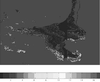
Figure 6.15. Same as Figure 6.11 but for 2 October, 2001.

sea. It could be conjectured that the chl distribution captured by SeaWiFS on 7 April, 2001 (Figure 6.11) reflects exactly this stage in the sequence of the marine biological cycles.

The onset of ice and snow melting is pivotal for the development of the micro- algae community in the White Sea because it marks the beginning of the biological spring.

However, with a developing exhaustion of nutrients, the spring phytoplankton bloom gradually declines (which is clearly obvious from the data in Figure 6.12) to then be followed by a new phytoplankton bloom in mid-summer.

The exact timing of this phase is variable depending upon the weather patterns. Importantly, at this time of year, the area of algal bloom covers the entire central part of the sea and even extends to its north-eastern tracts. It is assumed that Figure 6.13 corresponds to this major burst of phytoplankton development.

In August, the abundance of phytoplankton in the offshore areas rapidly declines, still leaving rather enhanced concentrations of micro-algae in the southern bays, which still remain well warmed and continue to accommodate enough nutrients via river discharge. Figure 6.14 fits well in this stage of phytoplank- ton development and its spatial distribution.

In autumn, a new cycle of phytoplankton development is generally observed, the exact timing of increased intensity being highly dependent upon weather conditions. By the end of October, the phytoplankton growth is completed. Obviously, the spatial distribution given in Figure 6.15 is one of the stages of this final cycle.

Comparison of results of numerical modeling with the satellite observation data on the variations in phytoplankton abundance and distribution across the White Sea

The obtained sequence of phytoplankton cycling development in the White Sea was further compared with the results of ecological modeling. However, such a compar- ison can only be qualitative because the obtained satellite data are concentrations of chl, whereas the numerical simulations provide the phytoplankton biomass. The chl concentration and phytoplankton biomass are certainly interrelated quantities, but the concrete relationships are arealy and vegetatively season-specific.

Figures 6.16-6.18 exemplify three phases of the White Sea phytoplankton devel- opment. The left-hand sides of these figures are satellite data, whereas the right-hand sides present the simulation results conducted for 2001 and respective time periods. Figures 6.16-6.18 appear to be mutually consistent, although it would be unreason- able to expect a perfect coincidence of the retrieved and simulated space patterns: the ecological model was initiated for 1948 and run until 2001. Most naturally, over this time period even minor departures from the actual situations in the White Sea s hydrology, weather and light regimes, etc., are bound to inevitably result in inaccuracies.

With these reservations in mind, the data in Figures 6.16-6.18 compare remark- ably well. This can be considered as an experimental confirmation of the adequacy of the developed ecological model and the validity of forecasting made as a consequence.

Summing up, it is believed that the developed tool for processing satellite optical data and inferring temporal and spatial distributions of CPAs has proved to be successful and efficient for contributing to a multifaceted portrait of a water body whose optical status falls into the category of case II water.

2 4 6 8 10 12 14

Longitude (oE)

Figure 6.16. Qualitative comparison between the chl (µg l-1) spatial distribution obtained from a SeaWiFS image taken over the White Sea in early May, 2001 (left panel ) and the simulated phytoplankton biomass (mgN m-3) for the same time period and year (right panel ).

Additionally, the obtained experience gives solid evidence that the combination of simulation and satellite data can be highly useful for gaining more ample and versatile information about the targeted aquatic environment.

6.2 PATTERNS OF THERMO-HYDRODYNAMIC PROCESSES AND FIELDS FROM NOAA AVHRR DATA

6.2.1 Introduction

Despite the relatively long history of White Sea investigations, we still have little data on the mesoscale and synoptic variability of its thermodynamic fields, particularly in

estuaries and bays. Some effective ways to investigate such processes are provided by modern satellite remote sensing methods. Such methods, however, are not efficient enough for small estuaries with axial lengths of about 1 km (e.g., Kemskiy Bay). This is due to the low spatial resolution of the Advanced Very-High Resolution Radio- meter (AVHRR) sensor, mounted on satellites of the NOAA, Meteor, and MODIS series. However, in terms of its spatial and temporal resolutions, the AVHRR sensor is well suited for studies of large semi-enclosed water bodies, such as Dvinskiy, Mezenskiy, Onezhskiy, and Kandalakshskiy Bays. It is well known that mesoscale processes are the predominant ones in the formation of sea internal and external thermal exchanges, and govern both the patterns of distribution of chemical and biological parameters and the ecosystem functioning. Studies and monitoring of the White Sea with the use of NOAA AVHRR data, which are widely accessible and have been archived for more than 20 years, are very important. Mesoscale synoptic variability in marine thermodynamic fields registered at the atmosphere-water interface, can also be related to various eddies, fronts, and non-stationary structures such as upwelling, coherent structures, mushroom eddies, jet streams, and river outflows. These processes and phenomena are generally responsible for the spatial and temporal distribution of suspended matter and polluted waters across a marine water body. Apart from water temperature discontinuities, various thermo-hydrodynamic structures can be traced from the dynamic behavior of spatial and temporal distributions of suspended matter (especially in coastal regions) as well as ice fields. Utilization of satellite data in the infrared (IR) and visible ranges of the electromagnetic spectrum is widespread for the investigation of such processes. This allows studying the dynamic phenomena during both the period of navigation, as well as at the onset of the ice-free period. The latter is the most challenging for direct measurements from on board research vessels and buoys. The most promising method to investigate the aforementioned spatial patterns is the use of satellite images taken sequentially over the sea surface. In this case, it is possible to detect the patterns of formation, development, and dissipation of thermo-hydrodynamic processes and phenomena. Moreover, since the NOAA satellite visitation frequency is several hours, this provides an opportunity of detecting spatial and temporal variability of marine phenomena on mesoscale and synoptic scales.

6.2.2 Data and methods

The primary source of information is the NOAA AVHRR data. The sensor s spectral region ranges from the visible (channels 1 and 2 with the spectral bands 0.58-0.68 and 0.725-1.1 µm, respectively) to the IR (channels 3, 4, and 5 with the spectral bands 3.55-3.93, 10.5-11.5, and 11.5-12.5 µm, respectively). The surface spatial resolution varies between 0.8-1.1 km for different spectral bands.

The raw satellite data were calibrated according to the methods described below as well as to the procedures described by several authors (Lauritson et al., 1979; McClain et al., 1985). At the NWPI of the Karelian Research Center (KRC) of the Russian Academy of Sciences (RAS), there is an archive of digital images of the

White Sea taken in the visible and thermal IR spectral ranges for all seasons during 1983-2002. The data obtained in the AVHRR thermal IR channels during the day- time is significantly contaminated with radiation, which is atmospherically scattered and reflected at the sea surface toward the direction of the sensor s aperture.

For calibration and atmospheric correction of AVHRR images taken over the White Sea, we performed in the summertime periods of 2001 and 2002 a suite of shipborne in situ measurements in Onezhskiy Bay. The measurements were conducted from on board the NWPI R/V Ecolog, a SeaCat probe and IR radiometer being used to this end. The shipborne measurements were effected simultaneously (or rather quasi-simultaneously) with satellite overpasses (Figure 6.19). This approach allows us to both perform an atmospheric correction and evaluate the weather conditions, which is important for sea surface temperature (SST) measurements and determination of the influence exerted by the so-called skin effect (the presence of a surface film whose temperature differs from that of the bulk water) on the water surface retrieval results obtained from satellite data.

The downloaded AVHRR images were subjected to the following processing steps:

• Transformation and geometric correction of satellite images, calibration, atmo- spheric correction, flagging and masking clouds and land areas, and the conversion of station coordinates and temperature measurements into equal projections.

• Determination of the brightness temperature in different channels from the downloaded images at particular observation points, and optimization of the temperature calculation algorithm based on the concurrent/semi-concurrent field measurements.

• Data conversion into formats compatible with various software packages, and finally, calculation of the water temperature.

The correction and transformation of images were performed using the Erdas Imagine 8.5 software package following the method of control points . As a base map, we used a vector map of the White Sea on a 1 : 1,000,000 scale. Subsequently, we imported the processed images into the Idrisi GIS format for calibration and temperature calculation. All measurements were calibrated during the preparation of satellite images for the eventual analysis. The original images were stored as .tdf files. The radiance determined from the signal in channel 1 was computed as a linear function of the input data values:

Ei= Si C + Ii (6.14)

where Ei is the radiance in mW/(m2· sr · cm-1); C is the input value (ranging from 0 to 1,023 counts); and Siand Iiare, respectively, the scaled slope and intercept values. The scaled thermal channel slope is measured in mW/(m2· sr · cm-1) per count and the intercept is expressed in mW/(m2· sr · cm-1). The conversion of radiance data into brightness temperature is performed using the inverse version of Planck s

(b)

Figure 6.19. Spatial distribution of the mean SST as (a) measured by an infrared radiometer on board the NWPI R/V Ecolog and (b) retrieved from NOAA AVHRR data. Averaging was performed for the period 10-14 July, 2001.

radiation equation:

T (E) =

C2

( C 3 \ (6.15)

E

where T is the temperature (K) corresponding to radiance E; is the central wave number of the channel (cm-1); and C1 and C2 are constants (C1= 1.191 0659 x 10-5mW/(m2· sr · cm-4) and C2= 1.438 833 cm · K). Note that the temperatures obtained by this procedure are not corrected for atmospheric impact.

Using the Idrisi GIS software package we calibrated and calculated the radio- brightness temperature deduced from the AVHRR fourth and fifth channels for each transformed picture. A polynomial was used for such calculations. Finally, the calculations of surface water temperature have been conducted using the following parameterization:

T (BT4, BT5) =

C4n BT n +

C5n BT n +

C45nm BT n BT m + C

n n

n,m

4 5

(6.16)

T (BT4, BT5)= C4 BT4 + C5 BT5 + C45 BT4 BT5 + C (6.17)

The coefficients C4, C5, C45, and C in this polynomial depend on the principal parameters such as the time and season of the satellite overpass, level of water turbulence, atmospheric humidity, etc. Usually, two sets of the polynomial coeffi- cients are employed: for daytime and night-time. In order to decrease the systematic errors arising from temperature calculations with identical coefficients under various conditions, we developed some procedures to optimize the desired coefficients. This method is based on a comparison of the measured and retrieved temperature at a concrete station. Coefficients averaged over the entire image area were obtained after comparing them with temperatures measured at several stations. In order to convert the coordinates from a geographic to a metric system, ArcView software was used. Subsequently, the data stored in .shp format was imported into the Erdas Imagine GIS. Based on the conversion algorithms, the brightness data were calibrated and converted in the radio-brightness temperature. From a comparative analysis, it was found that temperatures measured in situ and determined from the shipborne radio- meter readings differed only insignificantly: just a few decimal fractions of a degree. The smallest error was attained when we used data recovered from daytime IR- radiometer measurements. Figure 6.20 shows a comparison of temperature

(b)

Figure 6.20. Comparison of the SST as (a) measured by an IR radiometer on board the NWPI R/V Ecolog and (b) retrieved from NOAA AVHRR.

observed from different measurements procedures (on-board IR-radiometer and

Probe ) and calculated from satellite data.

To mask the cloud-screened areas and land areas we used an algorithm of the iterative cluster analysis, where pixels of the image were classified as pixels of different types. To present the results and to facilitate the treatment of initial tem- perature data, the latter were rounded to integers and the data file was exported into

.tif format using the common palette therm1.pal.

Based on the procedures developed at the Institute of Space Research (IKI) RAS

(Lupyan et al., 1998), the water surface temperature for a multi-year period was calculated. Our analysis of the processed AVHHR data for summertime indicates that a thin skin layer is generated during evening hours, when the upper sea surface is not yet cooled enough. Thus, there is a discrepancy between the SST determinations from evening and daytime satellite data - a better fit is obtained for the daytime option.

6.2.3 Results of NOAA satellite data analysis

Annual and seasonal variability

Based on our analysis of NOAA images for a 20-year period, the following general- ization of characteristic patterns of water temperature distributions throughout the White Sea, caused by various thermodynamic processes and phenomena, can be made. With de-icing of the White Sea in May, there is a front located between the Gorlo and Bassein. A zone of cold water, developing due to an upwelling generated by tidal movements, establishes around the Solovetzkiy Archipelago. In June, there are certain regions with enhanced water surface temperature near the estuaries of the Severnaya Dvina and Onega Rivers. This is a clear frontal boundary displacing with time into the areas of Onezhskiy and Dvinskiy Bays. During late July-early August, this zone of an increased water surface temperature encompasses practically the entire Dvinskiy Bay and the major part of Onezhskiy Bay. Contemporaneously, the frontal zones in Dvinskiy Bay and the Gorlo frequently merge into a single one. Small, but detectable temperature rises occur during that period, attributable to warming of bulk water in the inner part of Kandalakshskiy Bay. The increase in temperature due to river inflow is less detectable there than it is in Dvinskiy and Onezhskiy Bays. Finally, during September and October, the water surface tempera- ture is leveled in the bays and the Bassein. However, the frontal zones surrounding the Solovetzkiy Archipelago and the Gorlo persist through autumn.

Mesoscale and synoptic variability

Satellite images in the thermal IR reveal a significant mesoscale variability in the White Sea surface temperature. Real life distributions of water surface temperature can be appreciably different from the climatic patterns described earlier. During the sub-satellite INCO-Copernicus experiment conducted between 7-14 July, 2001, an increase of water surface temperature in the shallow area of the south-western coast of Onezhskiy Bay was revealed. This area becomes warmer during the first-half of the summer. Marine regions with maximal temperatures (> 18-19oC) are found near the estuaries of the Onega, Nigni Vig, and Kem Rivers, which discharge significant amounts of warm water during that time of year into the White Sea. Understand- ably, river discharge areas are not only regions of warm water, but also regions of low salinity.

The lowest temperature in this period (< 8oC) in the upper 5-m water layer was observed to the south and to the east off the Solovetzkiy Archipelago. This is thought to be due to penetration into this area of cold and relatively saline water

(> 270) from the Bassein through the Solovetzkiy Salma Strait and also owing to the upwelling of cold water caused by tidal movements (Semenov and Luneva, 1999). During that time, intensive water mixing is taking place off the Solovetzkiy Archipelago straits. Judging by the observed water temperature and salinity profiles, a relatively uniform mass of cold water establishes to the south off the Solovetzkiy Archipelago (Figure 4.10). The observed specific features of spatial distribution of water temperature and salinity data provide a basis for the assump- tion that water masses from the Bassein move into Onezhskiy Bay at this time of year, and is explained by relatively stable water dynamics. This is substantiated by the available field data on tidal movements as well as by modeling data on the residual water circulation (Neelov and Savchuk, 2003). During autumn, the patterns of thermohaline distribution, observed in spring, generally persist. However, the horizontal gradients became significantly less pronounced. Satellite images taken in July, 2001 display a strip (6-10 km wide) of relatively cold water with the surface temperature about 6-7oC. This strip was found along the Zimny coast off the Veprevskiy Cape. This elongated area of cold water was eventually generated by Ekman coastal upwelling.

In addition to the front in the Gorlo, all satellite images taken during summer- time displayed a front in Dvinskiy Bay - formed by the warm waters of the bay and cold waters coming from the Bassein. This front stretched from the Letny to the Zimny coasts at a distance of about 50 km from the estuary of the Dvina River. Importantly, this feature of water mass division is dynamically unstable, frequently transforming into separate jets (called also fingers ), invading the Bassein, and, in some cases, interacting with the frontal zone of the Gorlo Strait. The spatial scale of the jets reaches several tens of kilometers.

Our analysis of satellite images in the IR and visible ranges elucidated the nature and temporal behavior of jet currents, numerous mesoscale cyclonic and anticyclone eddies, coherent structures similar to mushroom eddies, as well as certain disconti- nuities related to Ekman coastal upwelling (Figure 6.21, see color section). Due to a high contrast between the warm and brackish river flows and water masses of the Basein (with gradients reaching 2oC km-1), the front in the Gorlo, as well as some frontal structures in Dvinskiy and Onezhskiy Bays are very distinctly discernible in the processed satellite images.

Data on the areas with developed coastal upwelling in the White Sea are in agreement with previous observations. These areas are associated with capes and/ or other relief specific features. For instance, the upwelling develops during various seasons around the Solovetzkiy Archipelago. According to Semenov et al. (1999) its development is promoted by regular tidal movements. Satellite images taken in summer over the area located off the eastern Solovetzkiy Salma reveal a quasi- permanent zone with a decreased SST (!it - 9oC), which is attributable to an intense frontal upwelling. Eddies were discovered off the Kandalakshskiy coast. The spatial scale of anticyclonic eddies is generally about 50 km. The anticyclonic eddies, frequently located between the Basein and Kandalakshskiy Bay, appear as a dipole with a relatively small (about 20 km) cyclonic eddy located on its periphery. During wintertime, such dynamic phenomena as mesoscale eddies, mushroom-

associated eddies, and circulations may be good indicators of ice cover state and dynamics. For the case of the White Sea, this indication is particularly valuable for the springtime, when the main ice cover is in a state of disintegration (Figure 6.22, see color section). The visible-band AVHRR data are well suited for monitoring ice fields. AVHRRR data from the winter and spring have depicted development of eddies of about 20 km in diameter near the edge of ice field disintegration (Figure 6.22).

The possible causal mechanism of development of these phenomena could be an instability arising from a discontinuity of horizontal currents in the near ice zone. Temporal changes in the development of these anticyclonic eddies could not be followed from space, due to heavy and highly frequent cloudiness - overcast con- ditions account for more than 190 days per year in the area of the White Sea. Therefore, it would be advantageous to use all-weather satellite images provided by synthetic aperture radar (SAR). The sequence of stages of ice cover disintegration and transfer of ice floes through the Gorlo to Voronka and further to the Barents Sea is shown in Figure 6.22 (see color section). A very fast disintegration of the ice is observed in the vicinity of estuaries, which are the main source of warm water entering the sea. This is also noticeable in the area of the Solovetzkiy Archipelago constituting the most active dynamic zone of the White Sea.

6.2.4 Discussion and main findings

Satellite data in the visible and IR reveal a diversity of water movements in the White Sea, ranging from large-scale circulation, encompassing vast regions of the sea, to a variety of quasi-permanent mesoscale or synoptic structures. These particular features are primarily responsible for spatial and temporal variations of the thermal (at least surficial) conditions in the White Sea. Figures 6.23 (see color section) and 6.24 summarize the types of water circulation obtained as a result of satellite image analyses. The characteristic features include eddies - monopoles, seen in SST spatial distributions (Figure 6.25), as well as in the dynamics of ice cover (Figure 6.26); dipoles (Figure 6.26(a, b)), jet currents (Figure 6.26(c)), mushroom eddies (Figure 6.26(d)), and structures due to front meandering (Figure 6.26(e)).

Relatively large-scale eddies (of a few tens of kilometers in diameter) were most often observed in the open parts of the Bassein at a 10-20 km distance off the Kola coast. Jet currents and mushroom eddies were found near the frontal areas. In general, however, such coherent structures should not be different by their tempera- ture from the ambient water. Possibly, such types of water movements as jet trans- frontal streams and frontal meandering (Figure 6.24) are in fact just different stages in the development of particular coherent structures. The basis for the evolution of such phenomena could be the deceleration of the jet current, initially appearing due to a relatively powerful local impulse. Such an impulse could be due to a diversity of causes: persistent wind stress in the open sea, differences in the level (and pressure), instability of fronts and currents, river discharge accompanied by wind in the coastal areas, features of local morphometry and general patterns of coastal circulation or water exchange through the straits, and tidal and inflow movements. In this

(a) 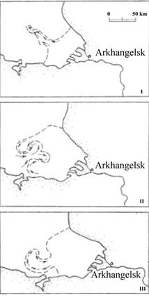(b)

Figure 6.24. Types of mesoscale and synoptic water circulation patterns in the White Sea as revealed by NOAA images: (a) I - anticyclonic eddy near the ice border (ice serves as a tracer), II - non-stationary dipole and monopole structures in the Bassein (water temperature serves as a tracer); (b) I - jet or trans-frontal stream in Dvinskiy Bay, II - mushroom-like eddies in Dvinskiy Bay, III - frontal meandering. Arrows indicate the direction of water movement.

Filatov and Shilov (1996).

particular case (Figure 6.24(c-e)), the possible mechanism for the development of mushroom eddies could be instability of the front in Dvinskiy Bay caused by transgression of cold water, this process being facilitated by tidal currents coming from the region of Solovetzkiy Salma.

Based on the analysis of sequential satellite IR images, spanning a several-day period, we have revealed significant spatial and temporal variability of SST fields over the entire White Sea. The maximum variability was observed in the proximity of frontal zones of Onezhskiy, Dvinskiy, and other large bays.

As it was emphasized above, the actual SST distribution across the White Sea could differ significantly from its climatic pattern. There is a clear need to combine

Figure 6.25. RADARSAT SAR image of the White Sea and the adjacent part of the Barents Sea taken on 28 February, 1998.

satellite observations in the IR, visible, and SAR data as well as in situ measurements from research vessels in order to better understand the mechanisms of formation and evolution of eddies, and various coherent structures that significantly alter the water regime in the White Sea. A comparative analysis of the combination of research vessel observations, AVHRR, and SeaWiFS data seems to be especially promising for attaining greater insight into the specific features of the thermo-hydrodynamics of the White Sea.

Date: 2016-03-03; view: 655