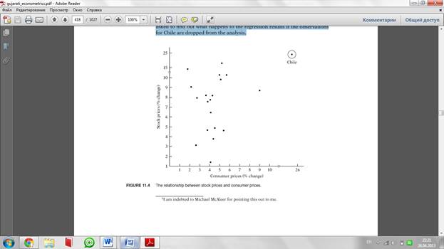
Heteroscedasticity can also arise as a result of the presence of outliers.

An outlying observation, or outlier, is an observation that is much different

(either very small or very large) in relation to the observations in the

sample. More precisely, an outlier is an observation from a different population

to that generating the remaining sample observations.3 The inclusion

or exclusion of such an observation, especially if the sample size is small,

can substantially alter the results of regression analysis.

As an example, consider the scattergram given in Figure 11.4. Based on the

data given in exercise 11.22, this figure plots percent rate of change of stock

prices (Y) and consumer prices (X) for the post–WorldWar II period through

1969 for 20 countries. In this figure the observation on Y and X for Chile can

be regarded as an outlier because the given Y and X values are much larger

than for the rest of the countries. In situations such as this, it would be hard

to maintain the assumption of homoscedasticity. In exercise 11.22, you are

asked to find out what happens to the regression results if the observations

for Chile are dropped from the analysis.

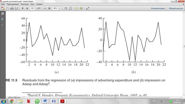
5.Another source of heteroscedasticity arises from violating Assumption

9 of CLRM, namely, that the regression model is correctly specified.

Although we will discuss the topic of specification errors more fully in

Chapter 13, very often what looks like heteroscedasticity may be due to the

fact that some important variables are omitted from the model. Thus, in the

demand function for a commodity, if we do not include the prices of commodities

complementary to or competing with the commodity in question

(the omitted variable bias), the residuals obtained from the regression may

give the distinct impression that the error variance may not be constant. But

if the omitted variables are included in the model, that impression may

disappear.

As a concrete example, recall our study of advertising impressions retained

(Y) in relation to advertising expenditure (X). (See exercise 8.32.) If

you regress Y on X only and observe the residuals from this regression, you

will see one pattern, but if you regress Y on X and X2, you will see another

pattern, which can be seen clearly from Figure 11.5. We have already seen

that X2 belongs in the model. (See exercise 8.32.)

6.Another source of heteroscedasticity is skewnessin the distribution

of one or more regressors included in the model. Examples are economic

variables such as income, wealth, and education. It is well known that the

distribution of income and wealth in most societies is uneven, with the bulk

of the income and wealth being owned by a few at the top.

7.Other sources of heteroscedasticity: As David Hendry notes, heteroscedasticity

can also arise because of (1) incorrect data transformation

(e.g., ratio or first difference transformations) and (2) incorrect functional

form (e.g., linear versus log–linear models).4

Note that the problem of heteroscedasticity is likely to be more common

in cross-sectional than in time series data. In cross-sectional data, one

usually deals with members of a population at a given point in time, such as

individual consumers or their families, firms, industries, or geographical

subdivisions such as state, country, city, etc. Moreover, these members may

be of different sizes, such as small, medium, or large firms or low, medium,

or high income. In time series data, on the other hand, the variables tend to

be of similar orders of magnitude because one generally collects the data for

the same entity over a period of time. Examples are GNP, consumption

expenditure, savings, or employment in the United States, say, for the period

1950 to 2000.

As an illustration of heteroscedasticity likely to be encountered in crosssectional

analysis, consider Table 11.1. This table gives data on compensation

per employee in 10 nondurable goods manufacturing industries, classified

by the employment size of the firm or the establishment for the year

1958. Also given in the table are average productivity figures for nine

employment classes.

17)What happens to ordinary least squares estimators and their variances in the presence of heteroscedasticity? (pp. 393–394, 442)

1.Following the error-learning models, as people learn, their errors of behavior

become smaller over time. In this case, σ2 i is expected to decrease.

2.As incomes grow, people have more discretionary income2 and hence

more scope for choice about the disposition of their income. Hence, σ2

i is likely to increase with income. Thus in the regression of savings on income

one is likely to find σ2 i increasing with income because people have more choices about their savings behavior.

Date: 2016-01-14; view: 1028