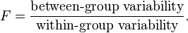
Give a definition for a T test, F test, G test.

A t-test is any statistical hypothesis test in which the test statistic follows a Student's t distribution if the null hypothesis is supported. It can be used to determine if two sets of data are significantly different from each other, and is most commonly applied when the test statistic would follow a normal distribution if the value of a scaling term in the test statistic were known. When the scaling term is unknown and is replaced by an estimate based on the data, the test statistic (under certain conditions) follows a Student's t distribution.

Among the most frequently used t-tests are:

· A one-sample location test of whether the mean of a population has a value specified in a null hypothesis.

· A two-sample location test of the null hypothesis such that the means of two populations are equal. All such tests are usually called Student's t-tests, though strictly speaking that name should only be used if the variances of the two populations are also assumed to be equal; the form of the test used when this assumption is dropped is sometimes called Welch's t-test. These tests are often referred to as "unpaired" or "independent samples" t-tests, as they are typically applied when the statistical units underlying the two samples being compared are non-overlapping.^[6]

· A test of the null hypothesis that the difference between two responses measured on the same statistical unit has a mean value of zero. For example, suppose we measure the size of a cancer patient's tumor before and after a treatment. If the treatment is effective, we expect the tumor size for many of the patients to be smaller following the treatment. This is often referred to as the "paired" or "repeated measures" t-test:^[6][7] see paired difference test.

· A test of whether the slope of a regression line differs significantly from 0.

An F-test is any statistical test in which the test statistic has an F-distribution under the null hypothesis. It is most often used when comparing statistical models that have been fitted to a data set, in order to identify the model that best fits the population from which the data were sampled. Exact "F-tests" mainly arise when the models have been fitted to the data using least squares. The name was coined by George W. Snedecor, in honour of Sir Ronald A. Fisher. Fisher initially developed the statistic as the variance ratio in the 1920s.

Most F-tests arise by considering a decomposition of the variability in a collection of data in terms of sums of squares. The test statistic in an F-test is the ratio of two scaled sums of squares reflecting different sources of variability. These sums of squares are constructed so that the statistic tends to be greater when the null hypothesis is not true. In order for the statistic to follow the F-distribution under the null hypothesis, the sums of squares should be statistically independent, and each should follow a scaled chi-squared distribution. The latter condition is guaranteed if the data values are independent and normally distributed with a common variance.

The formula for the one-way ANOVA F-test statistic is

or

In statistics, G-tests are likelihood-ratio or maximum likelihood statistical significance tests that are increasingly being used in situations where chi-squared tests were previously recommended.

The general formula for G is

where O_i is the observed frequency in a cell, E_i is the expected frequency under the null hypothesis, where ln denotes the natural logarithm and the sum is taken over all non-empty cells.

G-tests are coming into increasing use, particularly since they were recommended at least since the 1981 edition of the popular statistics textbook by Sokal and Rohlf.^[1]

Given the null hypothesis that the observed frequencies result from random sampling from a distribution with the given expected frequencies, the distribution of G is approximately a chi-squared distribution, with the same number of degrees of freedom as in the corresponding chi-squared test.

For very small samples the multinomial test for goodness of fit, and Fisher's exact test for contingency tables, or even Bayesian hypothesis selection are preferable to the G-test

The commonly used chi-squared tests for goodness of fit to a distribution and for independence in contingency tables are in fact approximations of the log-likelihood ratio on which the G-tests are based. The general formula for Pearson's chi-squared test statistic is

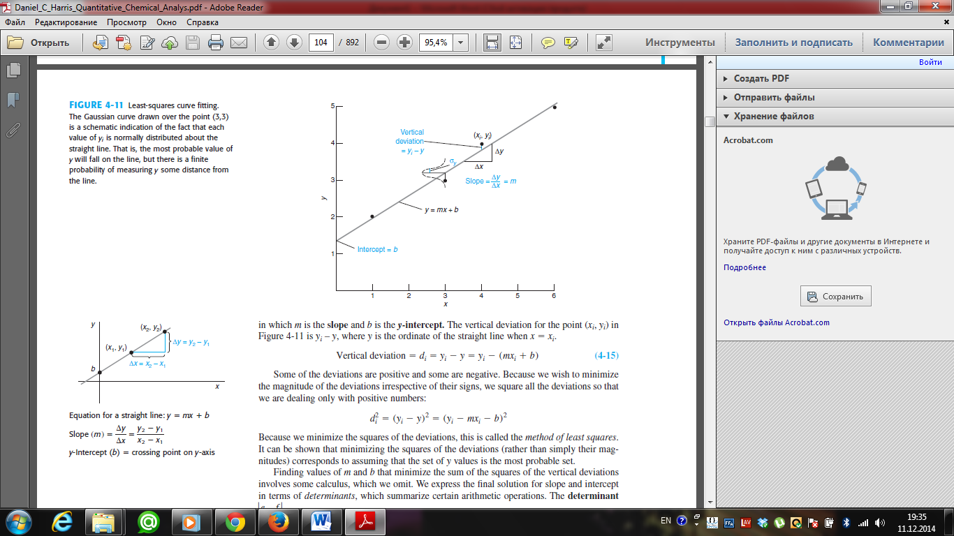
17. Explain the method of least squares.

For most chemical analyses, the response of the procedure must be evaluated for known quantities of analyte (called standards) so that the response to an unknown quantity can be interpreted. For this purpose, we commonly prepare a calibration curve. We use the method of least squares to draw the “best” straight line through experimental data points that have some scatter and do not lie perfectly on a straight line. The best line

will be such that some of the points lie above and some lie below the line.

Finding the Equation of the Line

The procedure we use assumes that the errors in the y values are substantially greater than the errors in the x values. This condition is often true in a calibration curve in which the experimental response (y values) is less certain than the quantity of analyte (x values). A second assumption is that uncertainties (standard deviations) in all y values are similar.

Equation of straight line: y = mx + b, in which m is the slope and b is the y-intercept. The vertical deviation for the point (xi, yi) in Figure-1 is yi – y, where y is the ordinate of the straight line when x = xi.

Finding values of m and b that minimize the sum of the squares of the vertical deviations involves some calculus, which we omit. We express the final solution for slope and intercept in terms of determinants, which summarize certain arithmetic operations.

The slope and the intercept of the “best” straight line are found to be

and n is the number of points.

18. What is the random error. Give an example.

Every measurement has some uncertainty, which is called experimental error. Conclusions can be expressed with a high or a low degree of confidence, but never with complete certainty. Experimental error is classified as either systematic or random.

Systematic error, also called determinate error, arises from a flaw in equipment or the design of an experiment. If you conduct the experiment again in exactly the same manner, the error is reproducible. In principle, systematic error can be discovered and corrected, although

this may not be easy. For example, a pH meter that has been standardized incorrectly produces a systematic error.

Suppose you think that the pH of the buffer used to standardize the meter is 7.00, but it is really 7.08. Then all your pH readings will be 0.08 pH unit too low. When you read a pH of 5.60, the actual pH of the sample is 5.68. This systematic error could be discovered by using a second buffer of known pH to test the meter.

Random error, also called indeterminate error, arises from uncontrolled (and maybe uncontrollable) variables in the measurement. Random error has an equal chance of being

positive or negative. It is always present and cannot be corrected. There is random error associated with reading a scale. Different people reading the scale in Figure 3-1 report a range of values representing their subjective interpolation between the markings. One person reading the same instrument several times might report several different readings. Another random error results from electrical noise in an instrument. Positive and negative fluctuations occur with approximately equal frequency and cannot be completely eliminated.

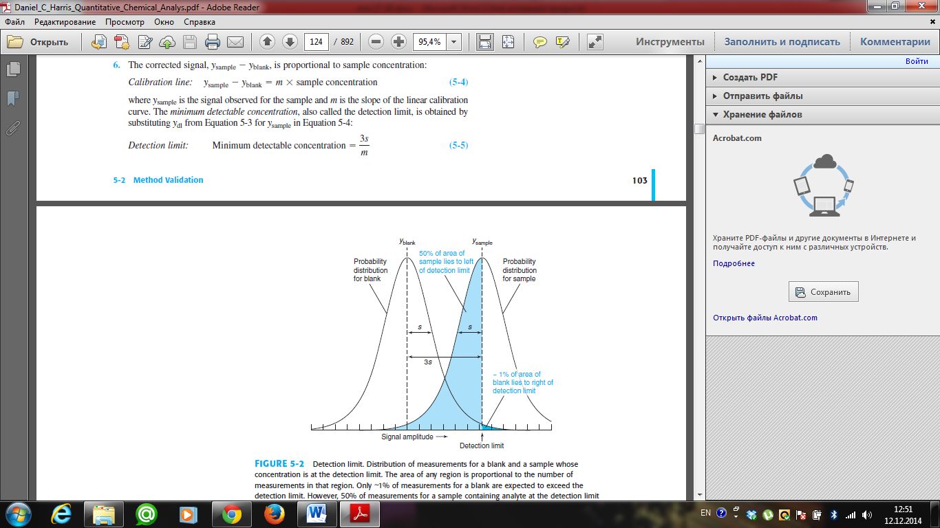
19. Explain and give the definitions to the following: calibration schedules, sensitivity coefficient, the lower bound of defined contents, detection limit.

A calibration curve is a general method for determining the concentration of a substance in an unknown sample by comparing the unknown to a set of standard samples of known concentration. A calibration curve is one approach to the problem of instrument calibration; other approaches may mix the standard into the unknown, giving an internal standard. A calibration curve shows the response of an analytical method to known quantities of analyte.

A spectrophotometer measures the absorbance of light, which is proportional to the quantity of substance analyzed. Solutions containing known concentrations of analyte are called standard solutions. Solutions containing all reagents and solvents used in the analysis, but no deliberately added analyte, are called blank solutions. Blanks measure the response of the analytical procedure to impurities or interfering species in the reagents.

The detection limit (also called the lower limit of detection) is the smallest quantity of analyte that is “significantly different” from the blank. Here is a procedure that produces a detection limit with chance of being greater than the blank. That is, only of samples containing no analyte will give a signal greater than the detection limit (Figure 5-2). We say that there is a rate of false positives in Figure 5-2. We assume that the standard deviation of the signal from samples near the detection limit is similar to the standard deviation from blanks.

Minimum detectable concentration = 3s/m

m - is the slope of the linear calibration curve, s- standard deviation

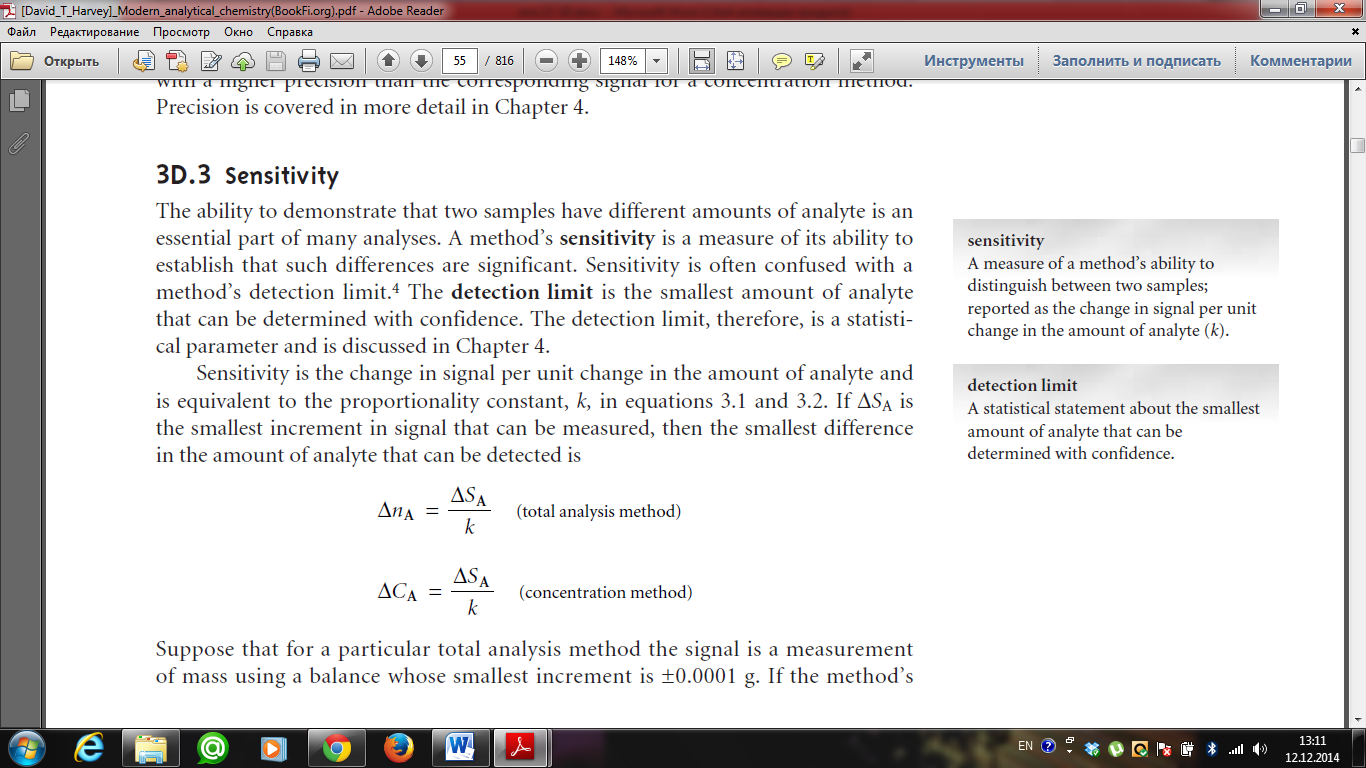
The lower limit of detection is 3s/m, where s is the standard deviation of a low-concentration sample and m is the slope of the calibration curve. The standard deviation is a measure of the noise (random variation) in a blank or a small signal. When the signal is 3 times greater than the noise, it is detectable, but still too small for accurate measurement. A signal that is 10 times greater than the noise is defined as the lower limit of quantitation( also called the lower bound of defined contents) or the smallest amount that can be measured with reasonable accuracy.

Lower limit of quantitation= 10s/m

Sensitivity

Sensitivity - the ability to demonstrate that two samples have different amounts of analyte is an essential part of many analyses. A method’s sensitivity is a measure of its ability to establish that such differences are significant. Sensitivity is often confused with a method’s detection limit. The detection limit is the smallest amount of analyte that can be determined with confidence.

Sensitivity is the change in signal per unit change in the amount of analyte and is equivalent to the proportionality constant, k. If ∆SA is the smallest increment in signal that can be measured, then the smallest difference in the amount of analyte that can be detected is

Suppose that for a particular total analysis method the signal is a measurement of mass using a balance whose smallest increment is ±0.0001 g. If the method’s sensitivity is 0.200, then the method can conceivably detect a difference of as little as

in the absolute amount of analyte in two samples.

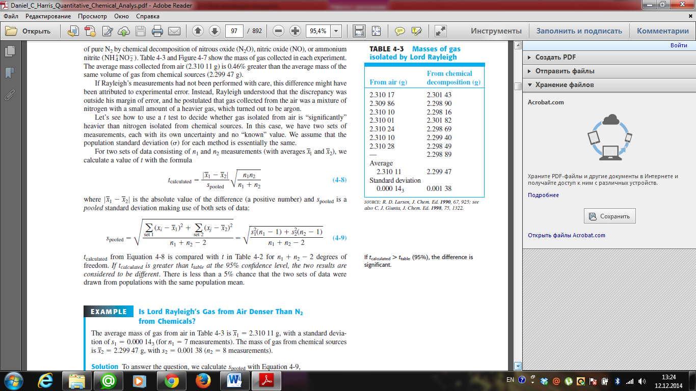
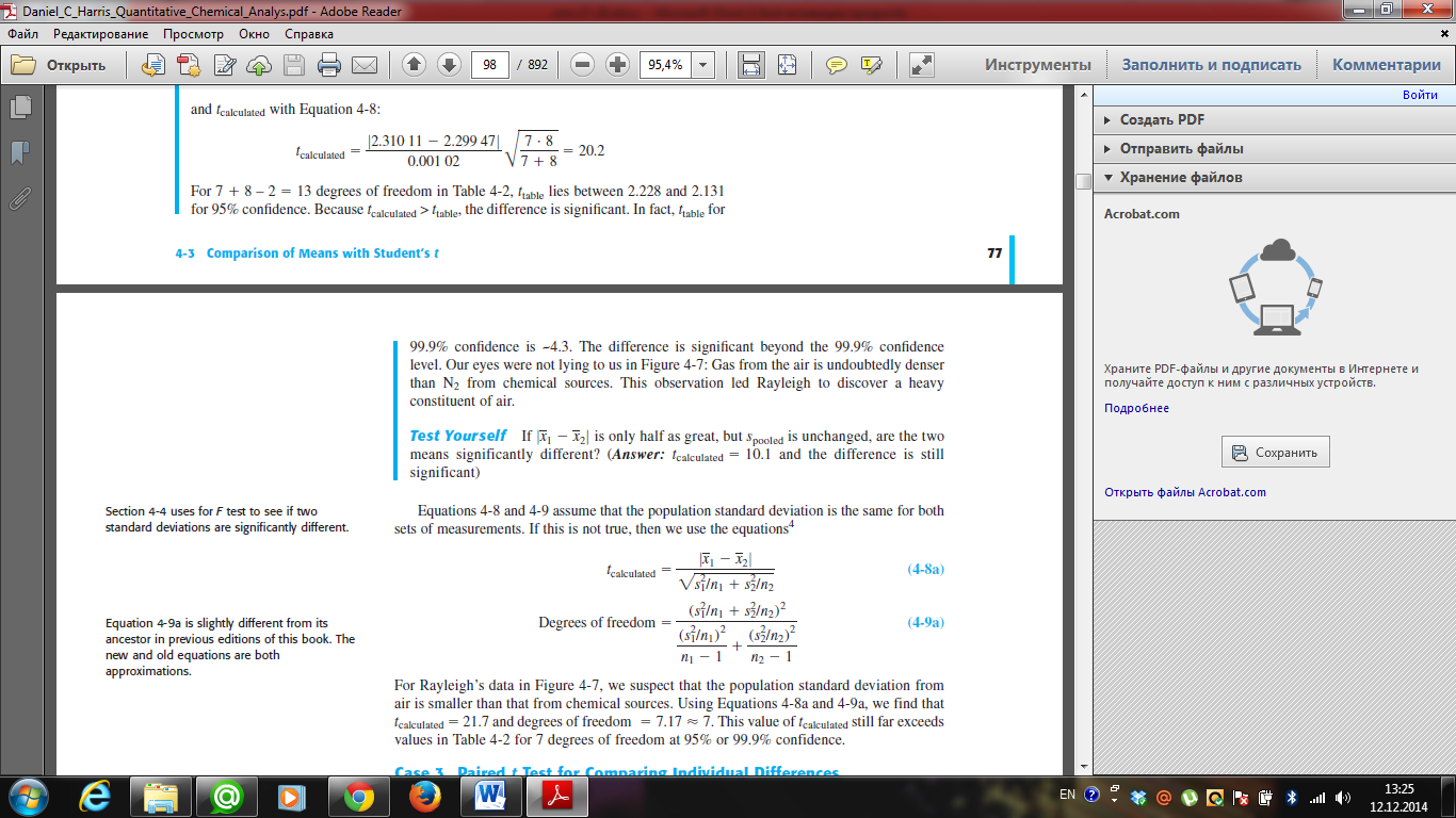
20. Explain comparison of dispersions. Describe the Fischer’s criterion.

If the standard deviations of two data sets are not significantly different from each other, then we use Equation 4-8 for the t test.

If the standard deviations are significantly different, then we use Equation 4-8a instead.

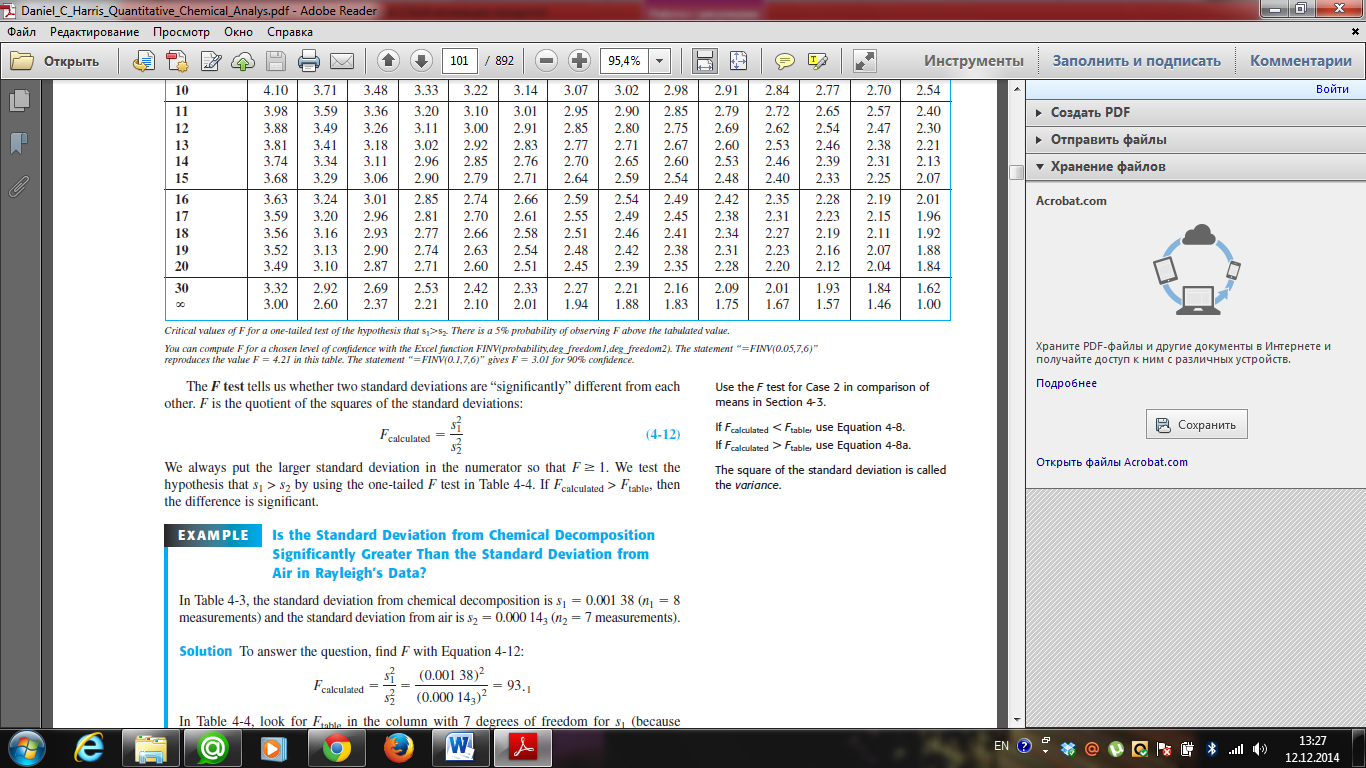
The F test tells us whether two standard deviations are “significantly” different from each

other. F is the quotient of the squares of the standard deviations:

We always put the larger standard deviation in the numerator so that F≥1. We test the hypothesis that s1 > s2

by using the one-tailed F test using critical values of F at 95% confidence level. If Fcalculated > Ftable, then

the difference is significant.

Date: 2016-01-14; view: 1463