CATEGORIES:
BiologyChemistryConstructionCultureEcologyEconomyElectronicsFinanceGeographyHistoryInformaticsLawMathematicsMechanicsMedicineOtherPedagogyPhilosophyPhysicsPolicyPsychologySociologySportTourism
c. Graphically identify the optimal cost-minimizing level of capital and labor in the long run if the firm wants to produce 140 units.
This is point C on the graph above. When the firm is at point B they are not minimizing cost. The firm will find it optimal to hire more capital and less labor and move to the new lower isocost line. All three isocost lines above are parallel and have the same slope.
D. If the marginal rate of technical substitution is , find the optimal level of capital and labor required to produce the 140 units of output.
Set the marginal rate of technical substitution equal to the ratio of the input costs so that 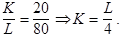 Now substitute this into the production function for K, set q equal to 140, and solve for L:
 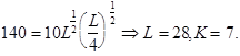 The new cost is TC=$20*28+$80*7 or $1120.
12. A computer company’s cost function, which relates its average cost of production AC to its cumulative output in thousands of computers Q and its plant size in terms of thousands of computers produced per year q, within the production range of 10,000 to 50,000 computers is given by
AC = 10 - 0.1Q + 0.3q.
A. Is there a learning curve effect?
The learning curve describes the relationship between the cumulative output and the inputs required to produce a unit of output. Average cost measures the input requirements per unit of output. Learning curve effects exist if average cost falls with increases in cumulative output. Here, average cost decreases as cumulative output, Q, increases. Therefore, there are learning curve effects.
B. Are there economies or diseconomies of scale?
Economies of scale can be measured by calculating the cost-output elasticity, which measures the percentage change in the cost of production resulting from a one percentage increase in output. There are economies of scale if the firm can double its output for less than double the cost. There are economies of scale because the average cost of production declines as more output is produced, due to the learning effect.
C. During its existence, the firm has produced a total of 40,000 computers and is producing 10,000 computers this year. Next year it plans to increase its production to 12,000 computers. Will its average cost of production increase or decrease? Explain.
First, calculate average cost this year:
AC1= 10 - 0.1Q + 0.3q = 10 - (0.1)(40) + (0.3)(10) = 9.
Second, calculate the average cost next year:
AC2= 10 - (0.1)(50) + (0.3)(12) = 8.6.
(Note: Cumulative output has increased from 40,000 to 50,000.) The average cost will decrease because of the learning effect.
13. Suppose the long-run total cost function for an industry is given by the cubic equation TC = a + bQ + cQ2+ dQ3. Show (using calculus) that this total cost function is consistent with a U-shaped average cost curve for at least some values of a, b, c, d.
To show that the cubic cost equation implies a U-shaped average cost curve, we use algebra, calculus, and economic reasoning to place sign restrictions on the parameters of the equation. These techniques are illustrated by the example below.
First, if output is equal to zero, then TC = a, where a represents fixed costs. In the short run, fixed costs are positive, a > 0, but in the long run, where all inputs are variable a = 0. Therefore, we restrict a to be zero.
Next, we know that average cost must be positive. Dividing TC by Q:
AC = b + cQ + dQ2.
This equation is simply a quadratic function. When graphed, it has two basic shapes: a U shape and a hill shape. We want the U shape, i.e., a curve with a minimum (minimum average cost), rather than a hill shape with a maximum.
At the minimum, the slope should be zero, thus the first derivative of the average cost curve with respect to Q must be equal to zero. For a U-shaped AC curve, the second derivative of the average cost curve must be positive.
The first derivative is c + 2dQ; the second derivative is 2d. If the second derivative is to be positive, then d > 0. If the first derivative is equal to zero, then solving for c as a function of Q and d yields: c = -2dQ. If d and Q are both positive, then c must be negative: c < 0.
To restrict b, we know that at its minimum, average cost must be positive. The minimum occurs when c + 2dQ = 0. We solve for Q as a function of c and d:  . Next, substituting this value for Q into our expression for average cost, and simplifying the equation:
 , or
, or
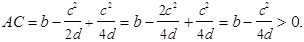
implying  . Because c2>0 and d > 0, b must be positive.
In summary, for U-shaped long-run average cost curves, a must be zero, b and d must be positive, c must be negative, and 4db > c2. However, the conditions do not insure that marginal cost is positive. To insure that marginal cost has a U shape and that its minimum is positive, using the same procedure, i.e., solving for Q at minimum marginal cost  and substituting into the expression for marginal cost b + 2cQ + 3dQ2, we find that c2must be less than 3bd. Notice that parameter values that satisfy this condition also satisfy 4db > c2, but not the reverse.
For example, let a = 0, b = 1, c = -1, d = 1. Total cost is Q - Q2+ Q3; average cost is
1 - Q + Q2; and marginal cost is 1 - 2Q + 3Q2. Minimum average cost is Q = 1/2 and minimum marginal cost is 1/3 (think of Q as dozens of units, so no fractional units are produced). See Figure 7.13.

Figure 7.13
*14. A computer company produces hardware and software using the same plant and labor. The total cost of producing computer processing units H and software programs S is given by
TC = aH + bS - cHS,
where a, b, and c are positive. Is this total cost function consistent with the presence of economies or diseconomies of scale? With economies or diseconomies of scope?
There are two types of scale economies to consider: multiproduct economies of scale and product-specific returns to scale. From Section 7.5 we know that multiproduct economies of scale for the two-product case, SH,S, are
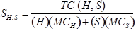
where MCHis the marginal cost of producing hardware and MCSis the marginal cost of producing software. The product-specific returns to scale are:
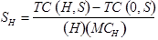 and
and
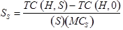
where TC(0,S) implies no hardware production and TC(H,0) implies no software production. We know that the marginal cost of an input is the slope of the total cost with respect to that input. Since

we have MCH= a - cS and MCS= b - cH.
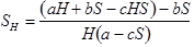
Substituting these expressions into our formulas for SH,S, SH, and SS:
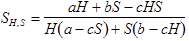 or
or
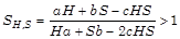 , because cHS > 0. Also,
 , or
, or
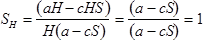 and similarly

There are multiproduct economies of scale, SH,S> 1, but constant product-specific returns to scale, SH= SC= 1.
Economies of scope exist if SC> 0, where (from equation (7.8) in the text):
 , or,
, or,
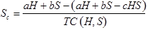 , or
, or

Because cHS and TC are both positive, there are economies of scope.
Date: 2015-12-24; view: 1672
| <== previous page | | | next page ==> |
| B. If the company produced 100,000 units of goods, what is its average variable cost? | | |