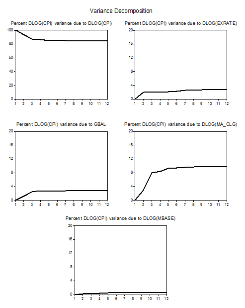
Variance Decomposition

[1] See, for instance, Walsh (1998, 138-157).

[2] We may have the same insight into why growth of money supply drives inflation, if we turn to quantity theory of money that relates nominal income, velocity of money and the money supply: where PY stands for nominal GDP (price level times real GDP), V denotes velocity of money, and M is the stock of money. If we assume that V and Y changes are relatively small over time, then proportionality between money and prices implies that persistent growth of money supply leads to a proportional rise in price level, i.e. to inflation.

[3] Following Sachs and Larrain (1993).

[4]

[5] However, there exists an alternative view on the problem. Ricardian Equivalence Hypothesis stresses that the borrowing is just deferred taxation. Reduction in taxes is surely to increase current fiscal deficit and therefore requires borrowing. But economic agents are rational and they anticipate future tax increases that the government would need to pay off its debts. That is why they in fact increase current private savings in order to compensate fully for additional future tax burden. In pure formulation, as advocated by Robert Barro (1989), a given tax cut and a fall in government saving will be exactly offset by growth of private savings so that all these pressures allegedly stemming from bond financing of budget deficit simply will not happen: interest rates won’t rise, private sector won’t crowd out etc. It should be noted that empirical evidence doesn’t support the presence of Ricardian Equivalence in developing world and is rather inconclusive as far as developed countries are concerned.

[6] This phenomenon was observed and documented for many Latin America countries.

[7] See Act of Verkhovna Rada (Ukrainian Parliament) “On Structure of the Budget Classification”, July, 12, 1996, # 327

[8] According to the IMF (1999) deficit consist of the following items: (1) total net treasury bill sales (total funds raised net of total interest repayment); (2) other net banking system credit to government (all non-treasury-bill financing extended to the budget by banks less all government deposits in the banking system); (3) receipts from privatisation; (4) all credit guaranteed by the government; (5) net proceeds from bonds issued by local authorities for the purpose of financing deficits of the consolidated budget; (6) net proceeds from bonds issued by the government to non-residents for deficit financing: (7) the difference between disbursements of foreign credits to the consolidated budget and the amortization of foreign credits by the consolidated budget; (8) the decline in government deposits in non-resident banks.

[9] See HIID (1999).

[10] In contrast, the money-dominant regime would show that the inflation depends only on money supply, so it is the monetary phenomena only.

[11] In other words, it is near impossible to find out which shocks are permanent, and which are temporary.

[12] We still expect some long-run relationship between money and prices to hold. This is to be the subject for a closer examination, but is beyond the scope of this paper.

[13] In addition, the following mnemonics are used: LOG denotes logarithm of the variable, HF denotes HPF filter, SA denotes Seasonally Adjusted by X-11.2 series, D denotes the first different, D(X,2) denotes the first difference.

[14] The interpretation of the impulse response functions (IRF) graphs is that they demonstrate dynamic responses of the inflation change to innovations in other variables.

[15] The dynamic semi-log elasticity (Pindyk and Rubienfeld, 1998) is calculated following the formula .

[16] To get the dynamic impact multiplier in terms of GDP, we multiplied the coefficient from the model by an average monthly GDP. The average monthly GDP over the period 1995:1-2000:6 was 8545 mln UAH. The coefficient, obtained directly from the model, answers the question: how disinflationary is a 1 mln UAH cut of the deficit?

[17] The exchange rate change seems to be highly inflationary during the first 3 months after the shock, but later on it is being compensated.

Date: 2015-02-28; view: 1228