Points of Clarification

i. AD and AS versus Demand and Supply Curves. It may be worthwhile the clarify the distinction between the AD and AS curves and the demand and supply curves from microeconomics. The AD curve plots the combinations of P and Y consistent with simultaneous equilibrium in the goods and financial markets. It slopes down because of the effect of P on the real money supply, and hence on the interest rate, investment, and output. It does not slope down because a lower price level makes goods more attractive to people. The AS curve plots the combinations of P and Y consistent with equilibrium in the labor market, conditional on the expected price level. It slopes up because higher output implies a lower unemployment rate and therefore a higher wage and therefore a higher price level. It does not slope up because firms desire to supply more goods when the price level is higher.

ii. Analysis of Shocks in the AD-AS Model. This is a difficult chapter. Students are likely to feel overwhelmed, particularly by the dynamics. To help students navigate the analysis of shocks in the AD-AS framework, instructors might wish to reinforce the steps in the analysis. Here is one possible outline:

a. Unless stated otherwise, assume that the economy begins in medium-run equilibrium. This implies that output is at its natural level, unemployment is at its natural rate, and the price level equals the expected price level.

b. Determine whether the shock affects the natural rate of unemployment. If the shock is to a variable in the IS-LM model, it will not affect the natural rate of unemployment. If the

Figure 7.3: An Oil Price Increase in the AD-AS Model

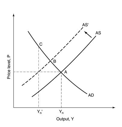
shock is to a variable in the AS curve (other than the price level or the expected price level), it will affect the natural rate of unemployment and thus the natural level of output.

c. Determine the initial shifts in the AD-AS diagram and IS-LM diagram. Do not neglect the secondary shift in the IS-LM diagram because of the change in price in the AD-AS diagram.

d. Determine whether the price level is greater than its expected level or less than its expected level. If the economy begins in medium-run equilibrium, the expected price level is the initial price level.

e. If the price level is greater than its expected level, then the AS curve will shift up over time until it intersects the (possibly new) AD curve at the (possibly new) natural level of output. Likewise, as the price level increases over time, the LM curve will shift up until it intersects the (possibly new) IS curve at the (possibly new) natural level of output. If the price level is less than its expected level, the AS and LM curves will shift down.

It is also useful to emphasize, as suggested in Chapter 6 of the Instructor's Manual, that the short-run, medium-run distinction is an analytical aid to help economists analyze the effects of shocks occurring at some point in time. In the real world, the economy is always experiencing some short-run shock and responding to previous shocks. The medium-run equilibrium describes a point to which the economy will tend to return in the absence of further shocks. The actual path of the economy, however, will depend on the sequence of shocks it receives.

Iii. Price Adjustment and Short-Run Equilibrium. Chapters 3 to 5 discussed the short run in the context of a fixed price level. In this chapter, the short-run equilibrium is the intersection of the AD and AS curves. Prices are allowed to change in the short run. Students may find this confusing. The IS-LM model adopts a fixed price assumption as a simplification. As this chapter shows, what is true in the short run is that prices may not adjust fully to restore the natural level of output, and more generally, that the actual price level may not equal the expected price level. Going deeper, the fundamental assumption is that nominal wages do not adjust to actual prices but to expected ones. This makes sense if wages are set for some period of time, so that wage setters base their decisions on expected prices over the life of the wage contract. On the other hand, wages are allowed to adjust immediately to changes in the unemployment rate, conditional on the expected price level. Such wage adjustment accounts for shifts along the AS curve in the short run. Clearly, a fully specified model would need to be careful about the terms and timing of wage adjustment. The AS framework in the text is a simplification intended to illustrate some basic issues—in particular slow price adjustment—at a manageable level of complexity.

Iv. The Natural Rate Hypothesis. Instructors may wish to say more about the natural rate hypothesis, as described in the context of the AD-AS model, and to explain the relationship between this hypothesis and the assumptions imposed in this chapter. The natural rate hypothesis typically has three elements. First, a natural rate exists, i.e., when the price level equals its expected price level (or when inflation equals expected inflation in a model with money growth), there is a unique unemployment rate consistent with labor market equilibrium. In the context of the model developed in Chapter 6 (in which the wage setting relation implies a negative relationship between nominal wages and the unemployment rate), the existence of a natural rate is guaranteed by the assumption that wages (in the wage setting relation) are proportional to expected prices. Second, the economy tends to return to the natural rate after shocks. In the AD-AS model, this result is generated by the assumption that the expected price level adapts to the history of the actual price level, i.e., when the actual price level is greater (less) than the expected price level, the price level expected in the future increases (decreases). Finally, the natural rate is reasonably stable, in the sense that it does not change so rapidly that economists can never measure it. Although the first two parts of the hypothesis could hold even if the natural rate changed very rapidly, the usefulness of the natural rate as a policy guide would be limited if it could not be measured with any confidence.

As will become clear in Chapter 8, the main evidence in the United States for the first two parts of the natural rate hypothesis is that the unemployment rate has a significant negative relationship with the change in the inflation rate. The benchmark empirical specification (with the change in the inflation rate on the LHS of a regression) incorporates two assumptions—that wage inflation is proportional to expected price inflation (i.e., that a natural rate exists) and that expected price inflation equals lagged price inflation. In reality, expectations formation is not all that well understood. At a minimum, expectations probably include some forward-looking elements. The text also notes that the natural rate can change over time and that relatively little is known about the determinants of the natural rate. Even if one accepts the stability of the U.S. natural rate since the 1970s, conventional techniques do not estimate it with much precision.

In sum, the natural rate hypothesis provides a powerful, unifying conceptual framework, but economists’ understanding of labor market equilibrium remains limited.

2. Alternative Sequencing

Chapter 13, which examines technological change and labor markets, includes a discussion of the effects of technological change on the AD-AS diagram. Instructors could present that part of Chapter 13 in the lecture on Chapter 7.

Date: 2015-02-16; view: 940