FORMING OF THE PRICE EXPECTATIONS

As you noticed, the prices of financial assets are determined by expectations of investors.

The generalizing formula is:

(4.5)

when Pr – current and past prices;

– expected changes in National income;

– expected changes in production costs.

The forming of price expectations is both backward and forward looking process.

Expectations formed by looking back are called adaptive expectations. This experience is measured as a weighted average of past values because the recent past (say, the last one to two years) is more significant than the more distant past. Thus, recent years are weighted more heavily than earlier years.

For example, if the rate of inflation has been 10 % per year for 7 years and fell down to 8 % in the most recent 2 years, the expected inflation rate in the coming year will be closer to 8 than to 10 percent.

It is clearly that expectations of future prices can’t be based only on last experience. Expectations formed by looking both backward and forward using all available information, are called rational expectations.

The theory of rational expectations states that expectations of financial prices on average are equal to the optimal forecast. The optimal forecast is the best guess possible arrived at by using all available information both from the past and about the future.

But even if a forecast is rational, there is no guarantee that the forecast will be accu­rate.

At first, there may be one or more additional key factors that are relevant but not available at the time the opti­mal forecast is made. If the information is not available, then the forecast may be inaccurate. However, it is still rational because the decision maker uses all available information.

At second, there are lags between the time that information becomes available and when it is fully incorporated into expectations. For example, as soon as market participants have come to better understand the process of inflation thanks to publications of Central Banks, the lag in adjusting expectations has sufficiently shortened.

Thus, in any given time period, it is possible to predict that the forecast error (or the difference between the actual value and the forecast) will exist. But on average it will be zero.

The efficient markets hypothesis is built on the theory of rational expectations. Namely, when financial markets are in equilibrium, the prices of financial instruments reflect all readily available information. Financial markets are in equilibrium when the quantity de­manded of any security is equal to the quantity supplied of that security. Returns reflect only differences in risk and liquidity. In an efficient market, the optimal forecast of a security's price (made by using all available informa­tion) will be equal to the equilibrium price.

Let's look once again at the share of stock from the previous example.

Suppose that an equi­librium return is 8 percent after adjusting for risk and liquidity (6% expected return on bonds + 2% risk premium = 8%).

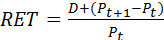
The return in terms of money in a given time period is equal to any dividend payment made during the time period plus the price of the stock at the end of the time period minus the price at the begin­ning of the time period. To express this return as a percentage, we need to divide the total return by the price at the beginning of the period, as in equation (4.2):

(4.6)

where D – dividend payments made during the period;

P_t – price at the beginning of the time period;

P_t+1 –price at the end of time period.

If at the beginning of the time period we know the price and dividend payment of the stock, then the only unknown variable is the price of the instrument at the end of the time period (P_t+1).

The efficient markets hypothesis assumes that the ex­pected or forecasted price of the stock at the end of the time period will be equal to the optimal forecast subject to using all available information. Thus, the exploring of the Equation (4.6) is suitable.

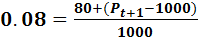Þ = 1000

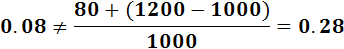
Let's assume now that Company-issuer announces new profit numbers that raise the expected price of the instrument at the end of the time period, for example, up to 1200 €.

The question is how today's price is respond to the new higher expected price in the future. Because having added new data in a formula we will receive an inequality:

Assuming that the risk and liquidity of the financial asset have not changed and that the equilibrium return (based on that risk and liquidity) of stock is 8 percent, the pre­sent price will adjust so that given the new expected price, the return will still be 8 percent.

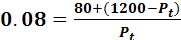Þ Solving for P_t Þ

Thus, the conclusion is that current price will rise to a level where the optimal forecast of an instrument's return is equal to the instrument's equilibrium return.

Thus, the current price will immediately rise to 1185.19 €, given the new higher expected price of 1200 €. When the current price is 1185.19 €, the expected return will be equal to 8 percent. At a price lower than 1185.19 €, the expected return would be higher. For example, at the original price of 1000 €, the expected return would be 28 per­cent.

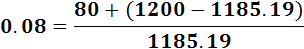
Funds would flow in this market by investors seeking the higher than equilibrium return of 8 percent based on risk and liq­uidity. As funds flowed in, the price of stock would rise. Funds would keep flowing into the market, pushing the price up until the market returned to equilibrium. This occurs at a price of 1185.19 because

The efficient markets hypothesis states that the prices of all financial instruments are based on the optimal forecast obtained by using all available information. A stronger version of the efficient markets hypothesis states that the prices of all financial instru­ments reflect the true fundamental value of the instruments. Thus, not only do prices reflect all available information but also this information is accurate, complete, under­stood by all, and reflects the market fundamentals. Market fundamentals are factors that have a direct effect on future income streams of the instruments. These factors include the value of the assets and the expected income streams of those assets on which the fi­nancial instruments represent claims.

Thus, if markets are efficient, prices are correct in that they represent underlying fundamentals. In the less-stringent version of the hypoth­esis, the prices of all financial instruments do not necessarily represent the fundamental value of the instrument.

There have been extraordinary run-ups and collapses of stock or bond prices, known as bubbles, which do not seem to be related to market fundamentals. Such run-ups in stock prices have occurred in Japan in the late 1980s and more recently in the United States in the late 1990s.

Some economists point out such bubbles in financial mar­kets can still be explained by rational expectations. It may be rational to buy a share of stock at a high price if it is thought that there will be other investors in the future who would be willing to pay inflated prices (prices that exceed those based on market funda­mentals) for the stock. This phenomenon is sometimes called "the greater fool" theory.

Other economists suspect that financial market prices may overreact before reach­ing equilibrium when there is a change in either supply or demand. That is, prices may rise or fall (overshoot or undershoot) more than market fundamentals would justify be­fore setting down to the price based on fundamentals. In these cases, it may be possible for investors to earn above average returns or to experience above average losses.

[1] Note that if you are not going to sell the stock the last summand is equal to zero, and n goes to infinity. To solve it for current price you need to set the limit of summation (for example it could be your expected age of surviving).

[2] Remind that the coefficient of a variation (CV) is a standardized measure of risk per unit of return:

, where – expected rate of return, – rate of return in scenario i, – probability of scenario i.

[3] Payments on bonds are made before payments to shareholders.

Date: 2014-12-22; view: 1225